Download
1 / 53
630 likes | 2.18k Views
Chapter 6 ~ Normal Probability Distributions. Chapter Goals. Learn about the normal , bell-shaped , or Gaussian distribution. How probabilities are found. How probabilities are represented. How normal distributions are used in the real world. 6.1 ~ Normal Probability Distributions.

E N D
Chapter Goals • Learn about the normal, bell-shaped, or Gaussian distribution • How probabilities are found • How probabilities are represented • How normal distributions are used in the real world
6.1 ~ Normal Probability Distributions • The normal probability distribution is the most important distribution in all of statistics • Many continuous random variables have normal or approximately normal distributions • Need to learn how to describe a normal probability distribution
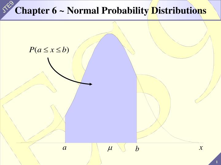
Normal Probability Distribution 3. Normal probability distribution function: This is the function for the normal (bell-shaped) curve - m 2 1 ( x ) 1 - = s 2 f ( x ) e s p 2 1. A continuous random variable 2. Description involves two functions: a. A function to determine the ordinates of the graph picturing the distribution b. A function to determine probabilities 4. The probability that x lies in some interval is the area under the curve
Probabilities for a Normal Distribution • Illustration
Notes • The definite integral is a calculus topic • We will use the TI83/84 to find probabilities for normal distributions • We will learn how to compute probabilities for one special normal distribution: the standard normal distribution • We will learn to transform all other normal probability questions to this special distribution • Recall the empirical rule: the percentages that lie within certain intervals about the mean come from the normal probability distribution • We need to refine the empirical rule to be able to find the percentage that lies between any two numbers
Percentage, Proportion & Probability • Basically the same concepts • Percentage (30%) is usually used when talking about a proportion (3/10) of a population • Probability is usually used when talking about the chance that the next individual item will possess a certain property • Area is the graphic representation of all three when we draw a picture to illustrate the situation
6.2 ~ The Standard Normal Distribution • There are infinitely many normal probability distributions • They are all related to the standard normal distribution • The standard normal distribution is thenormal distribution of the standard variable z(the z-score)
Standard Normal Distribution Properties: • The total area under the normal curve is equal to 1 • The distribution is mounded and symmetric; it extends indefinitely in both directions, approaching but never touching the horizontal axis • The distribution has a mean of 0 and a standard deviation of 1 • The mean divides the area in half, 0.50 on each side • Nearly all the area is between z = -3.00 and z = 3.00 Notes: • Table 3, Appendix B lists the probabilities associated with the intervals from the mean (0) to a specific value of z • Probabilities of other intervals are found using the table entries, addition, subtraction, and the properties above
Table 3, Appendix B Entries • The table contains the area under the standard normal curve between 0 and a specific value of z
Example • A portion of Table 3: z 0.00 0.01 0.02 0.03 0.04 0.05 0.06 . . . 1.4 0.4265 . . . • Example: Find the area under the standard normal curve between z = 0 and z = 1.45
Using the TI 83/84 • To find the area between 0 and 1.45, do the following: • 2ndDISTR 2 which is normalcdf( • Enter the lower bound of 0 • Enter a comma • Then enter 1.45 • Close the parentheses if you like or hit “Enter” • The value of .426 is shown as the answer! • Interpretation of the result: The probability that Z lies between 0 and 1.45 is 0.426
Example Area asked for • Example: Find the area under the normal curve to the right of z = 1.45; P(z > 1.45)
Using the TI 83/84 • To find the area between 1.45 and ∞, do the following: • 2ndDISTR 2 which is normalcdf( • Enter the lower bound of 1.45 • Enter a comma • Then enter 1 2nd EE 99 • Close the parentheses if you like or hit “Enter” • The value of .074 is shown as the answer! • Interpretation of result: The probability that Z is greater than 1.45 is 0.074
Example • Example: Find the area to the left of z = 1.45; P(z < 1.45)
Using The TI 83/84 • To find the area between - ∞ and 1.45, do the following: • 2ndDISTR 2 which is normalcdf( • Enter the lower bound of -1 2nd EE 99 • Enter a comma • Then enter 1.45 • Close the parentheses if you like or hit “Enter” • The value of 0.926 is shown as the answer! • Interpretation of result: The probability that Z is less than 1.45 is 0.926
Notes • The addition and subtraction used in the previous examples are correct because the “areas” represent mutually exclusive events • The symmetry of the normal distribution is a key factor in determining probabilities associated with values below (to the left of) the mean. For example: the area between the mean and z = -1.37 is exactly the same as the area between the mean and z = +1.37. • When finding normal distribution probabilities, a sketch is always helpful
Example Area asked for • Example: Find the area between the mean (z = 0) andz = -1.26
Using the TI 83/84 Area asked for - 0. 98 • Find the area to the left of z = -0.98 • Use -1E99 for - ∞ and enter 2nd DISTR • Normalcdf (-1e99, -0.98) which gives .164
Example - 2 . 30 1 . 80 - < < = - < < + < < P ( 2 . 30 z 1 . 80 ) P ( 2 . 30 z 0 ) P ( 0 z 1 . 80 ) = + = 0 . 4893 0 . 4641 0 . 9534 • Example: Find the area between z = -2.30 and z = 1.80
Using the TI 83/84 Find the area between z = -2.30 and z = 1.80 • Enter 2nd DISTR, normalcdf (-2.3, 1.80) and press enter • .953 is given as the answer. • Remember, the function normalcdf is of the form: • Normalcdf(lower limit, upper limit, mean, standard deviation) and if you’re working with distributions other than the standard normal (recall mean = 0, stddev = 1), you must enter the values for mean and standard deviation
Normal Distribution Note • The normal distribution table may also be used to determine a z-score if we are given the area (working backwards) • Example: What is the z-score associated with the 85th percentile?
Using the TI 83/84 • There is another function in the DISTR list that is used to find the value of z (or x) when the probability is given. For the previous problem, we are actually asking what is the value of z such that 85% of the distribution lies below it.
Using the TI 83/84 • Use 2ndDISTR invNorm( to calculate this value • 2ndDISTR invNorm(.85) “ENTER” gives us a value of 1.036 which is shown
Example • Example: What z-scores bound the middle 90% of a standard normal distribution?
Using the TI 83/84 • The TI 83/84 calculates areas from -∞ to the value of z we are interested in. Therefore, we must get a little creative to solve some problems. • Using the idea that the total area equals one comes in very handy here! • For the example given, where we are interested in the value of z that bounds the middle 90%, the tails therefore represent a total of 10%. Divide this in two since it is symmetric and this gives 5% in each tail.
Using the TI 83/84 • Now use the 2nd DISTR invNorm with .05 in the argument like this: • Which gives an answer of -1.645 • Since the distribution is symmetric, the upper limit is 1.645, so 90% of the distribution lies between (-1.645, 1.645)
Using the TI 83/84 Now let’s work the problems on page 279
6.3 ~ Applications of Normal Distributions • Apply the techniques learned for the z distribution to all normal distributions • Start with a probability question in terms ofx-values • Convert, or transform, the question into an equivalent probability statement involvingz-values
Standardization • The random variable has a standard normal distribution • Suppose x is a normal random variable with mean m and standard deviation s
Example Solutions: - m - 32.00 32.00 32.0 = = = = 1) When x 32.00 ; z 0.00 s 0.02 - m - 32.025 32 . 025 32.0 = = = = When x 32 . 025 ; z 1 . 25 s 0.02 • Example: A bottling machine is adjusted to fill bottles with a mean of 32.0 oz of soda and standard deviation of 0.02. Assume the amount of fill is normally distributed and a bottle is selected at random: 1) Find the probability the bottle contains between 32.00 oz and 32.025 oz 2) Find the probability the bottle contains more than 31.97 oz
Solution Continued Area asked for 32.0 - - - 32.0 32.0 x 32.0 32 . 025 32.0 æ ö < < = < < ç ÷ P ( 32.0 x 32 . 025 ) P è ø 0. 02 0. 02 0. 02 = < < = P ( 0 z 1 . 25 ) 0 . 3944
Example, Part 2 32.0 - 1 . 50 - - x 32.0 31 . 97 32.0 æ ö > = > = > - ç ÷ P ( x 31 . 97 ) P P ( z 1 . 50) è ø 0. 02 0. 02 = + = 0 . 5000 0 . 4332 0 . 9332 2)
Notes • The normal table may be used to answer many kinds of questions involving a normal distribution • Often we need to find a cutoff point: a value of x such that there is a certain probability in a specified interval defined by x • Example: The waiting time x at a certain bank is approximately normally distributed with a mean of 3.7 minutes and a standard deviation of 1.4 minutes. The bank would like to claim that 95% of all customers are waited on by a teller within c minutes. Find the value of c that makes this statement true.
Solution £ = P ( x c ) 0. 95 - - x 3 . 7 c 3 . 7 æ ö £ = ç ÷ P 0. 95 è ø 1 . 4 1 . 4 - c 3 . 7 æ ö £ = ç ÷ P z 0. 95 è ø 1 . 4
Example • Example: A radar unit is used to measure the speed of automobiles on an expressway during rush-hour traffic. The speeds of individual automobiles are normally distributed with a mean of 62 mph. Find the standard deviation of all speeds if 3% of the automobiles travel faster than 72 mph.
Solution > = P ( x 72 ) 0 . 03 > = P ( z 1 . 88 ) 0 . 03 - 72 62 1.88 = s s = = 10 / 1 . 88 5 . 32 - m x ; = z s 1 . 88 s = 10
Notation • If x is a normal random variable with mean m and standard deviation s, this is often denoted:x ~ N(m, s) • Example: Suppose x is a normal random variable with m= 35 and s = 6. A convenient notation to identify this random variable is: x ~ N(35, 6).
6.4 ~ Notation • z-score used throughout statistics in a variety of ways • Need convenient notation to indicate the area under the standard normal distribution • z(a) is the algebraic name, for the z-score (point on the z axis) such that there is a of the area (probability) to the right of z(a)
Illustrations z(0.10) represents the value of z such that the area to the right under the standard normal curve is 0.10 z(0.10) z(0.80) represents the value of z such that the area to the right under the standard normal curve is 0.80 z(0.80)
Example Table shows this area (0.4000) 0.10 (area information from notation) z(0.10) • Example: Find the numerical value of z(0.10): z(0.10) = 1.28
Example Look for 0.3000; remember that z must be negative z(0.80) • Example: Find the numerical value of z(0.80): • Use Table 3: look for an area as close as possible to 0.3000 • z(0.80) = -0.84
Notes • The values of z that will be used regularly come from one of the following situations: 1. The z-score such that there is a specified area in one tail of the normal distribution 2. The z-scores that bound a specified middle proportion of the normal distribution
Example 0.01 z(0.99) • Example: Find the numerical value of z(0.99): • Because of the symmetrical nature of the normal distribution, z(0.99) = -z(0.01)
Example z(0.995) z(0.005) -z(0.005) z(0.005) = 2.575 and z(0.995) = -z(0.005) = -2.575 • Example: Find the z-scores that bound the middle 0.99 of the normal distribution:
6.5 ~ Normal Approximation of the Binomial • Recall: the binomial distribution is a probability distribution of the discrete random variable x, the number of successes observed in n repeated independent trials • Binomial probabilities can be reasonably estimated by using the normal probability distribution
Background & Histogram 0.18 0.16 0.14 0.12 0.10 0.08 0.06 0.04 0.02 0.00 20 0 1 2 3 4 5 6 7 8 9 10 11 12 13 14 15 16 17 18 19 • Background: Consider the distribution of the binomial variable x when n = 20 and p = 0.5 • Histogram: The histogram may be approximated by a normal curve
Notes • The normal curve has mean and standard deviation from the binomial distribution: • Can approximate the area of the rectangles with the area under the normal curve • The approximation becomes more accurate as n becomes larger
Two Problems 1. As p moves away from 0.5, the binomial distribution is less symmetric, less normal-looking Solution: The normal distribution provides a reasonable approximation to a binomial probability distribution whenever the values of np and n(1 - p) both equal or exceed 5 2. The binomial distribution is discrete, and the normal distribution is continuous Solution: Use the continuity correction factor. Add or subtract 0.5 to account for the width of each rectangle.