Download
1 / 62
620 likes | 733 Views
The Financial Crisis and Macroeconomic Policy: Four Years On John B. Taylor Stanford University MONFISPOL Conference September 19, 2011. The Revival of Keynesian Discretionary Fiscal Policy in the 2000s. Economic Growth and Tax Relief Reconciliation Act of 2001

E N D
The Financial Crisis and Macroeconomic Policy: Four Years OnJohn B. TaylorStanford UniversityMONFISPOLConference September 19, 2011
The Revival of Keynesian Discretionary Fiscal Policy in the 2000s • Economic Growth and Tax Relief Reconciliation Act of 2001 • Refund checks; first installment of 2001 tax rate cuts • Economic Stimulus Act of 2008 (February) • Rebate checks and credits • American Recovery and Reinvestment Act of 2009 (February) • One-time payments, withholding change, refunds • More government spending too • Miscellaneous interventions in 2009-10 • Cash for clunkers program • First time home buyers program • Tax Relief , Unemployment Insurance Reauthorization, and Job Creation Act of 2010 (December)) • Temporary cut in payroll tax • American Jobs Act of 2011?
Keynesian Discretionary Fiscal Policy First Became Popular in the ‘60s & ‘70s • First in academia in the 1950s and 1960s • Arguments appeared in the major textbooks (Samuelson). • Keynesian econometric models • Then in practice: 1962 Economic Report of the President • “The task of economic stabilization cannot be left entirely to built-in stabilizers,” the report warned. “Discretionary budget policy, e.g. changes in tax rates or expenditure programs, is indispensible—sometimes to reinforce, sometimes to offset, the effects of the stabilizers.” • investment tax credit (1962), tax surcharge (1968) • tax rebates (1975) • countercyclical grants to states for infrastructure (1977-78) • Keynesian discretionary policy continued to the late 1970s.
Keynesian Policy Fell Out of Favorin ‘80s & ‘90s • Research raised doubts about discretionary policy • Lucas and Sargent “After Keynesian Economics” • Gramlich “the general idea of stimulating the economy through state and local governments is probably not a very good one” • Soon automatic stabilizers dominated the budget cycle • Bush 41: proposed tiny stimulus package in 1992 • Shift $10 billion in G from future to the present • did not pass the Congress • Clinton: proposed tiny stimulus in 1993 • $16 billion more G • did not pass the Congress. • Eichenbaum (1997) “there is now widespread agreement that countercyclical discretionary fiscal policy is neither desirable nor politically feasible.”
Original E line line New E I falls by this The Basic Model: A decline in I causes the aggregate expenditure line to shift down 25_10 SPENDING 45-degree line Original point of spending balance amount New point of spending balance Income or real GDP falls by this amount (more than by amount I falls ). INCOME OR REAL GDP New Original income income level level
G rises Countercyclical discretionary fiscal policy:Increase in G raises GDP depending on size of the multiplier and amount of crowding out 25_10 SPENDING 45-degree line INCOME OR REAL GDP
But Macro Models Differ Greatly • Romerand Bernstein (Jan 2009) used estimated old Keynesian models (without RE) to predict ARRA effect • Large multipliers, around 1.5. • Cogan, Cwik, Taylor and Wieland (Feb 2009) used estimated New Keynesian model to predict ARRA effect • Much smaller multipliers, around 0.5. • What not use these existing macro models for the evaluation of actual packages? • Because they simply repeat the same prediction story over again. • So you learn virtually nothing
A Stylized Illustration Consider two models relating stimulus S to output Y. Model A is Y= αS +Z Model B is Y = Z where Z is a shock and α =1.5 Now, suppose that a stimulus is enacted: S = 2 and Y decreases by -1 According to Model A ,Z = - 4 According to Model B, Z= -1 Now consider policy evaluation withcounterfactual: S=0 Economists using Model Asay: Just as we predicted, the stimulus package worked. Without it, Y would have fallen to -4 rather than -1. The decline in outputwould have been 4 times as deep, a Great Depression 2.0. Economists using Model Bsay Just as we predicted the stimulus package did not work.
A Less Stylized Illustration Robert Barro Harvard New Keynesian Smets - ECB “The accumulation of hard data and real-life experience has allowed more dispassionate analysts to reach a consensus that the stimulus package, messy as it is, is working” New York Times November 12, 2009
Use a Direct Approach • Micro data (used in 2001, 2008) • Shapiro and Slemrod (2003, 2009), • Johnson, Parker, Souleles (2006) • Parker, Souleles, Johnson, and McClelland (2009). • Macro data • Special BEA satellite account • “Personal Income and Output” (monthly to mid ’09) • “Effect of the ARRA on Selected Federal Government Sector Transactions” (quarterly)
Monthly Data on Rebate Payments in 2001 and 2008 ($ billions, annual rates) 20012008 April 0 23.3 May 0 577.1 June 0 334.4 July 95.1 164.1 August 223.1 12.4 September 144.9 0 October 2.5 0
Temporary stimulus meets • permanent income hypothesis
Temporary stimulus meets permanent income hypothesis again
Cash for clunkers: incentives really matter Based on Mian and Sufi (2010)
Quarterly PCE Regressions With and Without Stimulus Payments (1) (2) (3) Disposable Personal .817 ---- ----- Income (40.9) Disposable Personal Income--Without Stimulus ---- .857 .851 (73.0) (60.4) Stimulus Payments ----- ----- 0.128 (0.81) Oil Price ($/bbl lagged 2 quarters) -2.41 -2.55 -2.55 (-4.71) (-4.14) (-4.61) Net Worth (lagged 2 quarters) .021 .017 .018 (8.53) (7.32) (7.97) Standard error of regression 76.965.866.3
State and local government budget constraint • Gt + Et + Lt = Rt + At • where • G = Government purchases of goods and services • E = Expenditures other than for the purchases • L = Lending or borrowing (-), net • A= ARRA grants (exogenous) • R = Revenues excluding ARRA grants (exogenous) Estimated 3-equation system (1969Q1- 2011Q1) Gt = 3.86 + 0.864Gt-1+ 0.124Rt- 0.114At Et = -3.83+ 0.818Et-1 + 0.0398Rt+ 0.113At Lt = .0321 - 0.864Gt-1 - 0.818Et-1 + .836Rt + 1.001At
The Plausibility of the Counterfactual • Weren’t many states borrowing constrained after the crisis? • Not clear but in any case Fed’s Flow of Funds data show that that net borrowing would have increased even with such borrowing constraints. • Net borrowing = net increase in liabilities - net acquisition of financial assets • Net borrowing = - $118 billion from 2008 to 2010. Net increase in liabilities = $53 billion Net acquisition of financial assets = $171 billion. • Thus state and local government added significantly to their financial assets as ARRA grants came in. • With no ARRA they would not have done so.
Why the Negative Effect on Purchases? • “Other expenditures” consist largely of Medicaid, TANF, and other transfer programs • ARRA conditioned states’ receipt of additional Medicaid grants on their not reducing benefits or restricting eligibility rules • In some states, this meant undoing benefit reductions or eligibility restrictions that were implemented in the previous 6 months • July 1, 2008 is the date in Section 5001 of ARRA • This “hold-harmless” provision, may have forced states to reallocate funds that would have been used for purchases
Regressions with ARRA grants split into Medicaid (M) and other (N)
Net Effect on Federal, State& Local Government Purchases • If government purchases have a greater impact on GDP than temporary transfers—which the permanent income theory predicts—then ARRA could have had a negative effect • According to the simulations the cumulative negative effect on state and local government purchases was $85 billion (341/4). Larger than the $30 billion (119/4) cumulative positive effect of ARRA on federal government purchases.
Toward Discretion: ‘60s & ‘70s • Fed did not follow Milton Friedman’s rules message “of setting itself a steady course and sticking to it.” (AEA 1968) • 1965-1970s saw a series of boom-bust cycles in monetary policy with inflation rising steadily higher at each cycle. • The wage and price controls of the 1970s • Epitome of interventionist policy • Defended by Fed Chair Burns: “wage rates and prices no longer respond as they once did to the play of market forces.” • Insider reports showed little strategy or systematic thinking • Econometric studies show that Fed’s responses to inflation were unstable over time in the 1970s • Rising implicit inflation target • Not rule-like as it would become in the 1980s and 1990s.
1965-1980: monetary policy not well described by a rules-based price stability objective From “Has the Fed Gotten Tougher on Inflation?” The FRBSF Weekly Letter, March 31, 1995, by John P Judd and Bharat Trehan of the San Francisco Fed 1965-79
Toward Rules in the ‘80s –’90s • Dramatic shift of policy under Volcker in 1979-87. • Volcker (1983) “We have…gone a long way toward changing the trends of the past decade and more.” • Policy continued in ‘80s and ‘90s under Greenspan. • Additional evidence of more rules-based policy • more predictable and transparent decision-making process • focus on expectations of future policy actions. • announcing interest rate decisions when making them. • Transcripts of the FOMC in the 1990s, many references to rules. • Actual monetary policy closer to simple policy rule
Monetary policy gets more predictable, inflation targets, rules-based From “Has the Fed Gotten Tougher on Inflation?” The FRBSF Weekly Letter, March 31, 1995, by John P Judd and Bharat Trehan of the San Francisco Fed 1965-79 1987-92 1993-94
Illustrative monetary policy chart from St Louis Fed February 2007, Bill Poole
The Swing Away from Rules in Recent Years • Interest rates too low for too long in 2003-05 • On-again, off-again bailouts financed by central bank’s balance sheet • on for BSC creditors’ bailout, off for Lehman creditors’ bailout, on for AIG creditors’ bailout, off for TARP role out • Government regulators and supervisors deviated from sound regulatory rules, especially at large banks
Illustrative monetary policy chart from St Louis Fed February 2007, Bill Poole
Illustrative monetary policy chart from St Louis Fed February 2007, Bill Poole
Chart from Kansas City Fed, 2009, Tom Hoenig (2000-2009)