Download
1 / 28
440 likes | 1.5k Views
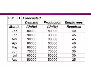
Chapter 12 – Independent Demand Inventory Management. Types of Inventory. Uses of Inventory. Anticipation or seasonal inventory Safety stock: buffer demand fluctuations Lot-size or cycle stock: take advantage of quantity discounts or purchasing efficiencies

E N D
Uses of Inventory • Anticipation or seasonal inventory • Safety stock: buffer demand fluctuations • Lot-size or cycle stock: take advantage of quantity discounts or purchasing efficiencies • Pipeline or transportation inventory • Speculative or hedge inventory protects against some future event, e.g. labor strike • Maintenance, repair, and operating (MRO) inventories
Inventory Management Objectives • Provide desired customer service level: • Percentage of orders shipped on schedule • Percentage of line items shipped on schedule • Percentage of dollar volume shipped on schedule • Idle time due to material and component shortages • Provide for cost-efficient operations: • Buffer stock for smooth production flow • Maintain a level work force • Allowing longer production runs & quantity discounts • Minimize inventory related investments: • Inventory turnover = Annual CGS/Avg Inv ($) • Weeks (or days) of supply = Avg Inv ($)/AvgWkUsage
Customer Service Level Examples • Percentage of Orders Shipped on Schedule • Good measure if orders have similar value. Does not capture value. • If one company represents 60% of your business but only 5% of your orders, 95% on schedule could represent only 40% of value • Percentage of Line Items Shipped on Schedule • Recognizes that not all orders are equal, but does not capture $ value of orders. More expensive to measure. OK for finish. goods. • A 90% service level might mean shipping 225 items out of the total 250 line items totaled from 20 orders scheduled • Percentage Of Dollar Volume Shipped on Schedule • Recognizes thedifferences inorders in terms of both line items and $ value
Inventory Investment Measures Example: The Coach Motor Home Company has annual cost of goods sold of $10,000,000. The average inventory value at any point in time is $384,615. Calculate inventory turnover and weeks/days of supply. • Inventory • Weeks/Days of Supply:
Three Mathematical Models for Determining Order Quantity • Economic Order Quantity (EOQ or Q System) • A model used to find optimal order q. and RP (Reorder Point) • Part of continuous review system which tracks on-hand inventory each time a withdrawal is made • Economic Production Quantity (EPQ) • A model that allows for incremental product delivery • Quantity Discount Model • Modifies the EOQ process to consider cases where quantity discounts are available
Economic Order Quantity • EOQ Assumptions: • Demand is known & constant - no safety stock is required • Lead time is known & constant • No quantity discounts are available • Ordering (or setup) costs are constant • All demand is satisfied (no shortages) • The order quantity arrives in a single shipment
Total Annual Inventory Cost with EOQ Model • Total annual cost= annual ordering cost + annual holding costs
Continuous (Q) Review System Example: A computer company has annual demand of 10,000. They want to determine EOQ for circuit boards which have an annual holding cost (H) of $6 per unit, and an ordering cost (S) of $75. They want to calculate TC and the reorder point (R) if the purchasing lead time is 5 days. • EOQ (Q) • Reorder Point (R) • Total Inventory Cost (TC)
Economic Production Quantity (EPQ) • Same assumptions as the EOQ except: inventory arrives in increments & is drawn down as it arrives
EPQ Equations • Total cost: • Maximum inventory: • d=demand rate • p=production rate • Calculating EPQ
Quantity Discount Model • Same as the EOQ, except: • Unit price depends upon the quantity ordered • Use the total cost equation:
Quantity Discount Procedure • Calculate the EOQ at the lowest price • Determine whether the EOQ is feasible at that price • Will the vendor sell that quantity at that price? • If yes, stop – if no, continue • Check the feasibility of EOQ at the next higher price • Continue to the next slide ...
QD Procedure (continued) • Continue until you identify a feasible EOQ • Calculate the total costs (including total item cost) for the feasible EOQ model • Calculate the total costs of buying at the minimum quantity required for each of the cheaper unit prices • Compare the total cost of each option & choose the lowest cost alternative • Any other issues to consider?
Quantity Discount Example: Collin’s Sport store is considering going to a different hat supplier. The present supplier charges $10 each and requires minimum quantities of 490 hats. The annual demand is 12,000 hats, the ordering cost is $20, and the inventory carrying cost is 20% of the hat cost. A new supplier is offering hats at $9 in lots of 4000. Who should he buy from? • EOQ at lowest price $9. Is it feasible? • Since the EOQ of 516 is not feasible, find the EOQ for the next lowest price -> EOQ = 490 (feasible). Compare 490 with 4,000. • 4000 hats at $9 each saves $19,320 annually. Space?
If demand or lead time is uncertain, safety stock can be added to improve order-cycle service levels R = d*L +SS Where SS =zσdL, and Z is the number of standard deviations and σdL is standard deviation of the demand during lead time Order-cycle service level The probability that demand during lead time will not exceed on-hand inventory A 95% service level (stockout risk of 5%) has a Z=1.645 Safety Stock and Service Levels
Periodic Review Systems • Orders are placed at specified, fixed-time intervals (e.g. every Friday), for a order size (Q) to bring on-hand inventory (OH) up to the target inventory (TI), similar to the min-max system. • Advantages are: • No need for a system to continuously monitor item • Items ordered from the same supplier can be reviewed on the same day saving purchase order costs • Disadvantages: • Replenishment quantities (Q) vary • Order quantities may not quality for quantity discounts • On the average, inventory levels will be higher than Q systems-more stockroom space needed
Periodic Review Systems: Calculations for TI • Targeted Inventory level: TI = d(RP + L) + SS d = average period demand RP = review period (days, wks) L = lead time (days, wks) SS = zσRP+L,where σRP+L= σ√RP+L • Replenishment Quantity (Q)=TI-OH
Periodic Review System: Annual demand (D) is 4160 units, avg. weekly demand is d = 80 units (4160/52), weekly σ is 1.77 units, and lead time is 3 weeks. H=$0.97 per unit per year, and S=$10 per order. • EOQ = √2DS/H = √2x4160x10/0.97 = 293 • Review Period RP = (EOQ/D) = (293/4160) = 0.07 year = 0.07 x 52 weeks = 3.66 weeks ~ 4 weeks • Target Inventory for 95% Service Level TI = d(RP + L)+zσRP+L, where σRP+L= σ√RP+L TI = 80(4 + 3) + 1.645*1.77√(4 + 3) = 560 + 7.70 = 567.70 ~ 568 Amount to order Q = TI- OH, where OH is the current inventory level (e.g., if OH = 324, Q = 568-324 = 244 units to order)
Single Period Inventory Model • The SPI model is designed for products that share the following characteristics • Sold at their regular price only during a single-time period • Demand is highly variable but follows a known probability distribution • Salvage value is less than its original cost so money is lost when these products are sold for their salvage value • Objective is to balance the gross profit of the sale of a unit with the cost incurred when a unit is sold after its primary selling period
SPI Model Example: Tee shirts are purchased in multiples of 10 for a charity event for $8 each. When sold during the event the selling price is $20. After the event their salvage value is just $2. From past events the organizers know the probability of selling different quantities of tee shirts within a range from 80 to 120 Payoff Table Prob. Of Occurrence .20 .25 .30 .15 .10 Customer Demand80 90 100 110 120 # of Shirts OrderedProfit 80 $960 $960 $960 $960 $960 $960 90 $900 $1080 $1080 $1080 $1080 $1040 Buy 100 $840 $1020 $1200 $1200 $1200 $1083 110 $780 $ 960 $1140 $1320 $1320 $1068 120 $720 $ 900 $1080 $1260 $1440 $1026 Sample calculations: Payoff (Buy 110)= sell 100($20-$8) –((110-100) x ($8-$2))= $1140 Expected Profit (Buy 100)= ($840 X .20)+($1020 x .25)+($1200 x .30) + ($1200 x .15)+($1200 x .10) = $1083
ABC Inventory Classification • ABC classification is a method for determining level of control and frequency of review of inventory items; Pr. 20. • A Pareto analysis can be done to segment items into value categories depending on annual dollar volume • A Items – typically 20% of the items accounting for 80% of the inventory value-use Q system • B Items – typically an additional 30% of the items accounting for 15% of the inventory value-use Q or P • C Items – Typically the remaining 50% of the items accounting for only 5% of the inventory value-use P
ABC Example: the table below shows a solution to an ABC analysis. The information that is required to do the analysis is: Item #, Unit $ Value, and Annual Unit Usage. The analysis requires a calculation of Annual Usage $ and sorting that column from highest to lowest $ value, calculating the cumulative annual $ volume, and grouping into typical ABC classifications.
Inventory Record Accuracy • Inaccurate inventory records can cause: • Lost sales • Disrupted operations • Poor customer service • Lower productivity • Planning errors and expediting • Two methods are available for checking record accuracy • Periodic counting-physical inventory • Cycle counting-daily counting of pre-specified items provides the following advantages: • Timely detection and correction of inaccurate records • Elimination of lost production time due to unexpected stock outs • Structured approach using employees trained in cycle counting