Presenting results from statistical models
Presenting results from statistical models. Professor Vernon Gayle and Dr Paul Lambert (Stirling University) Wednesday 1st April 2009. Structure of the Seminar. Should take 1 semester!!! Principals of model construction and interpretation Key variables – measurement and func. Form

Presenting results from statistical models
E N D
Presentation Transcript
Presenting results from statistical models Professor Vernon Gayle and Dr Paul Lambert (Stirling University) Wednesday 1st April 2009
Structure of the Seminar Should take 1 semester!!! • Principals of model construction and interpretation • Key variables – measurement and func. Form • Presenting results • Longitudinal data analysis • Individuals in households – multilevel models
“One of the useful things about mathematical and statistical models [of educational realities] is that, so long as one states the assumptions clearly and follows the rules correctly, one can obtain conclusions which are, in their own terms, beyond reproach. The awkward thing about these models is the snares they set for the casual user; the person who needs the conclusions, and perhaps also supplies the data, but is untrained in questioning the assumptions….
…What makes things more difficult is that, in trying to communicate with the casual user, the modeller is obliged to speak his or her language – to use familiar terms in an attempt to capture the essence of the model. It is hardly surprising that such an enterprise is fraught with difficulties, even when the attempt is genuinely one of honest communication rather than compliance with custom or even subtle indoctrination” (Goldstein 1993, p. 141).
Structure of the this session • Presenting results • This talk could also take weeks on end • Two topics only - not the final word • Quasi-Variances • Sample Enumeration methods • Many more topics emerging, • propensity score matching • simulation modelling
Using Quasi-variance to Communicate Sociological Results from Statistical Models Vernon Gayle & Paul S. LambertUniversity of Stirling Gayle and Lambert (2007) Sociology, 41(6):1191-1208
A little biography (or narrative)… • Since being at Centre for Applied Stats in 1998/9 I has been thinking about the issue of model presentation • Done some work on Sample Enumeration Methods with Richard Davies • Summer 2004 (with David Steele’s help) began to think about “quasi-variance” • Summer 2006 began writing a paper with Paul Lambert
The Reference Category Problem • In standard statistical models the effects of a categorical explanatory variable are assessed by comparison to one category (or level) that is set as a benchmark against which all other categories are compared • The benchmark category is usually referred to as the ‘reference’ or ‘base’ category
The Reference Category Problem An example of Some English Government Office Regions 0 = North East of England ---------------------------------------------------------------- 1 = North West England 2 = Yorkshire & Humberside 3 = East Midlands 4 = West Midlands 5 = East of England
Table 1: Logistic regression prediction that self-rated health is ‘good’ (Parameter estimates for model 1 )
Conventional Confidence Intervals • Since these confidence intervals overlap we might be beguiled into concluding that the two regions are not significantly different to each other • However, this conclusion represents a common misinterpretation of regression estimates for categorical explanatory variables • These confidence intervals are not estimates of the difference between the North West and Yorkshire and Humberside, but instead they indicate the difference between each category and the reference category (i.e. the North East) • Critically, there is no confidence interval for the reference category because it is forced to equal zero
Formally Testing the Difference Between Parameters - The banana skin is here!
Standard Error of the Difference Variance North West (s.e.2 ) Only Available in the variance covariance matrix Variance Yorkshire & Humberside (s.e.2 )
Standard Error of the Difference 0.0083 = Variance North West (s.e.2 ) Only Available in the variance covariance matrix Variance Yorkshire & Humberside (s.e.2 )
Formal Tests t = -0.03 / 0.0083 = -3.6 Wald c2 = (-0.03 /0.0083)2 = 12.97; p =0.0003 Remember – earlier because the two sets of confidence intervals overlapped we could wrongly conclude that the two regions were not significantly different to each other
Comment • Only the primary analyst who has the opportunity to make formal comparisons • Reporting the matrix is seldom, if ever, feasible in paper-based publications • In a model with q parameters there would, in general, be ½q (q-1) covariances to report
Firth’s Method (made simple) s.e. difference ≈
Firth’s Method (made simple) s.e. difference ≈ 0.0083 = t = (0.09-0.12) / 0.0083 = -3.6 Wald c2 = (-.03 / 0.0083)2 = 12.97; p =0.0003 These results are identical to the results calculated by the conventional method
Information from the Variance-Covariance Matrix Entered into the Data Window (Model 1) 0 0 0.00010483 0 0.00007543 0.00011543 0 0.00007543 0.00007543 0.00012312 0 0.00007543 0.00007543 0.00007543 0.00011337 0 0.00007544 0.00007543 0.00007543 0.00007543 0.00011480 0 0.00007545 0.00007544 0.00007544 0.00007544 0.00007545 0.00010268 0 0.00007544 0.00007543 0.00007544 0.00007543 0.00007544 0.00007546 0.00011802 0 0.00007552 0.00007548 0.00007550 0.00007547 0.00007554 0.00007572 0.00007558 0.00015002 0 0.00007547 0.00007545 0.00007546 0.00007545 0.00007548 0.00007555 0.00007549 0.00007598 0.00012356
Benefits Overcomes the reference category problem when presenting models Provides reliable results (even though based on an approximation) Easy(ish) to calculate Has extensions to other models Costs Extra column in results Time convincing colleagues that this is a good thing QV Conclusion – We should start using method
Example Drew, D., Gray, J. and Sime, N. (1992) Against the odds: The Education and Labour Market Experiences of Black Young People
Comparison of Odds Greater than 1 “higher odds” Less than 1 “lower odds”
Naïve Odds • In this model (after controlling for other factors) White pupils have an odds of 1.0 Afro Caribbean pupils have an odds of 3.2 • Reporting this in isolation is a naïve presentation of the effect because it ignores other factors in the model
Pupil with 4+ higher passes White Professional parents Male Graduate parents Two parent family Pupil with 0 higher passes Afro-Caribbean Manual parents Male Non-Graduate parents One parent family A Comparison
Odds are multiplicative 4+ Higher Grades 1.0 1.0 Ethnic Origin 1.0 3.2 Social Class 1.0 0.5 Gender 1.0 1.0 Parental Education 1.0 0.6 No. of Parents 1.0 0.9 Odds 1.0 0.86
Naïve Odds • Drew, D., Gray, J. and Sime, N. (1992) warn of this danger…. • …Naïvely presenting isolated odds ratios is still widespread (e.g. Connolly 2006 Brit. Ed. Res. Journal 32(1),pp.3-21) • We should avoid reporting isolated odds ratios where possible!
Generally, people find it hard to directly interpret results on the logit scale – i.e. b Logit scale
Log Odds, Odds, Probability • Log odds converted to odds = exp(log odds) • Probability = odds/(1+odds) • Odds = probability / (1-probability)
Log Odds, Odds, Probability Odds are asymmetric – beware!
Divide by 4 rule • Gelman and Hill (2008) suggest dividing coefficients from logit models by 4 as a guide for assessing the effects of the b estimated for a given explanatory variable as a probability • They assert that b/4 provides a ‘rule of convenience’ for estimating the upper bound of the predictive difference corresponding to a unit change in the explanatory variable. • Gelman and Hill (2008) are careful to report that this is an approximation and that it performs best near the midpoint of the logistic curve • We believe that this has some merit as a rough and ready method of interpreting the effects of estimates and is a useful tool especially when tables of coefficients are rapidly flashed up at a conference presentation Gelman, A. and J. Hill (2008) Data Analysis Using Regression and Multilevel/Hierarchical Models, Cambridge: Cambridge University Press
Communicating Results (to non-technically informed audiences) • Davies (1992) Sample Enumeration • Payne (1998) Labour Party campaign data • Gayle et al. (2002) • War against the uninformed use of odds (e.g. on breakfast t.v.)
Sample Enumeration Methods In a nutshell… “What if” – what if the gender effect was removed 1. Fit a model (e.g. logit) 2. Focus on a comparison (e.g. boys and girls) 3. Use the fitted model to estimate a fitted value for each individual in the comparison group 4. Sum these fitted values and construct a sample enumerated % for the group
Naïve Odds • Naïvely presenting odds ratios is widespread (e.g. Connolly 2006) • In this model naïvely (after controlling for other factors) Girls have an odds of 1.0 Boys have an odds of .58 We should avoid this where possible!
Logit Model • Example from YCS 11 (these pupils took GCSE in 2001) y=1 5+ GCSE passes (A* - C) X vars gender; family social class (NS-SEC); ethnicity; housing tenure; parental education; parental employment; school type; family type
Naïve Odds • Example from YCS 11 (these pupils took GCSE in 2001) • In this model naïvely (after controlling for other factors) Girls have an odds of 1.0 Boys have an odds of .66 We should avoid this where possible!
Pseudo Confidence Interval Bootstrapping to construct a pseudo confidence interval (1000 Replications)
Reference • A technical explanation of the issue is given in Davies, R.B. (1992) ‘Sample Enumeration Methods for Model Interpretation’ in P.G.M. van der Heijden, W. Jansen, B. Francis and G.U.H. Seeber (eds) Statistical Modelling, Elsevier We have recently written a working paper on logit models http://www.dames.org.uk/publications.html

