Download

1 / 43
430 likes | 522 Views
Lecture slides for Automated Planning: Theory and Practice. Chapter 17 Planning Based on Model Checking. Dana S. Nau Dept. of Computer Science, and Institute for Systems Research University of Maryland. c. a. b. Grasp block c. c. b. a. Intended outcome. a. b. c.

E N D
Lecture slides for Automated Planning: Theory and Practice Chapter 17Planning Based on Model Checking Dana S. Nau Dept. of Computer Science, and Institute for Systems Research University of Maryland
c a b Graspblock c c b a Intendedoutcome a b c Unintendedoutcome Motivation • Actions with multiple possibleoutcomes • Action failures • e.g., gripper drops its load • Exogenous events • e.g., road closed • Like Markov Decision Processes (MDPs),but without probabilities attached to the outcomes • Useful if accurate probabilities aren’t available, orif probability calculations would introduce inaccuracies
Nondeterministic Systems • Nondeterministic system: a triple = (S, A) • S = finite set of states • A = finite set of actions • : S A 2s • Like in the previous chapter, the book doesn’t commit to any particular representation • It only deals with the underlying semantics • Draw the state-transition graph explicitly • Like in the previous chapter, a policy is a function from states into actions • π: SA • At certain points we will also have nondeterministic policies • π: S 2A, or equivalently, π S A
Example • Robot r1 startsat location l1 • Objective is toget r1 to location l4 • π1 = {(s1, move(r1,l1,l2)), (s2, move(r1,l2,l3)), (s3, move(r1,l3,l4))} • π2 = {(s1, move(r1,l1,l2)), (s2, move(r1,l2,l3)), (s3, move(r1,l3,l4)), (s5, move(r1,l3,l4))} • π3 = {(s1, move(r1,l1,l4))} 2 Start Goal
Example • Robot r1 startsat location l1 • Objective is toget r1 to location l4 • π1 = {(s1, move(r1,l1,l2)), (s2, move(r1,l2,l3)), (s3, move(r1,l3,l4))} • π2 = {(s1, move(r1,l1,l2)), (s2, move(r1,l2,l3)), (s3, move(r1,l3,l4)), (s5, move(r1,l3,l4))} • π3 = {(s1, move(r1,l1,l4))} 2 Start Goal
Example • Robot r1 startsat location l1 • Objective is toget r1 to location l4 • π1 = {(s1, move(r1,l1,l2)), (s2, move(r1,l2,l3)), (s3, move(r1,l3,l4))} • π2 = {(s1, move(r1,l1,l2)), (s2, move(r1,l2,l3)), (s3, move(r1,l3,l4)), (s5, move(r1,l3,l4))} • π3 = {(s1, move(r1,l1,l4))} 2 Start Goal
Execution Structures s5 • Execution structurefor a policy π: • The graph of all ofπ’s execution paths • Notation: π = (Q,T) • QS • T S S • π1 = {(s1, move(r1,l1,l2)), (s2, move(r1,l2,l3)), (s3, move(r1,l3,l4))} • π2 = {(s1, move(r1,l1,l2)), (s2, move(r1,l2,l3)), (s3, move(r1,l3,l4)), (s5, move(r1,l3,l4))} • π3 = {(s1, move(r1,l1,l4))} 2 s2 s3 Start s1 s4 Goal
Execution Structures s5 • Execution structurefor a policy π: • The graph of all ofπ’s execution paths • Notation: π = (Q,T) • QS • T S S • π1 = {(s1, move(r1,l1,l2)), (s2, move(r1,l2,l3)), (s3, move(r1,l3,l4))} • π2 = {(s1, move(r1,l1,l2)), (s2, move(r1,l2,l3)), (s3, move(r1,l3,l4)), (s5, move(r1,l3,l4))} • π3 = {(s1, move(r1,l1,l4))} s2 s3 s1 s4
Execution Structures • Execution structurefor a policy π: • The graph of all ofπ’s execution paths • Notation: π = (Q,T) • QS • T S S • π1 = {(s1, move(r1,l1,l2)), (s2, move(r1,l2,l3)), (s3, move(r1,l3,l4))} • π2 = {(s1, move(r1,l1,l2)), (s2, move(r1,l2,l3)), (s3, move(r1,l3,l4)), (s5, move(r1,l3,l4))} • π3 = {(s1, move(r1,l1,l4))} 2 Start s1 s4 Goal
Execution Structures • Execution structurefor a policy π: • The graph of all ofπ’s execution paths • Notation: π = (Q,T) • QS • T S S • π1 = {(s1, move(r1,l1,l2)), (s2, move(r1,l2,l3)), (s3, move(r1,l3,l4))} • π2 = {(s1, move(r1,l1,l2)), (s2, move(r1,l2,l3)), (s3, move(r1,l3,l4)), (s5, move(r1,l3,l4))} • π3 = {(s1, move(r1,l1,l4))} s1 s4
s0 s3 a2 a0 s2 s1 Goal a1 Types of Solutions • Weak solution: at least one execution path reaches a goal • Strong solution: every execution path reaches a goal • Strong-cyclic solution: every fair execution path reaches a goal • Don’t stay in a cycle forever if there’s a state-transition out of it s0 s3 Goal a2 a0 s2 s1 Goal a3 a1 a3 s0 s3 a2 a0 Goal s2 s1 a1
Finding Strong Solutions • Backward breadth-first search • StrongPreImg(S) = {(s,a) : (s,a) ≠ ,(s,a) S} • all state-action pairs for whichall successors are in S • PruneStates(π,S) = {(s,a) π : s S} • S is the set of states we’vealready solved • keep only the state-actionpairs for other states • MkDet(π') • π' is a policy that may be nondeterministic • remove some state-action pairs ifnecessary, to get a deterministic policy
Example 2 π = failure π' = Sπ' = SgSπ'= {s4} Start s4 Goal
Example s5 2 π = failure π' = Sπ' = SgSπ'= {s5} PreImage = {(s3,move(r1,l3,l4)), (s5,move(r1,l5,l4))} π'' = {(s3,move(r1,l3,l4)), (s5,move(r1,l5,l4))} s3 Start s4 Goal
Example s5 2 π = failure π' = Sπ' = SgSπ'= {s5} PreImage = {(s3,move(r1,l3,l4)), (s5,move(r1,l5,l4))} π'' = {(s3,move(r1,l3,l4)), (s5,move(r1,l5,l4))} π = π' = {(s3,move(r1,l3,l4)), (s5,move(r1,l5,l4))} s3 Start s4 Goal
Example s5 2 π = π' = {(s3,move(r1,l3,l4)), (s5,move(r1,l5,l4))} Sπ' = {s3,s4,s5} SgSπ'= {s3,s4,s5} s3 Start s4 Goal
Example s5 2 s2 π = π' = {(s3,move(r1,l3,l4)), (s5,move(r1,l5,l4))} Sπ' = {s3,s4,s5} SgSπ'= {s3,s4,s5} PreImage = {(s2,move(r1,l2,l3)),(s3,move(r1,l3,l4)), (s5,move(r1,l5,l4)),(s4,move(r1,l4,l3)),(s4,move(r1,l4,l5))} π'' = {(s2,move(r1,l2,l3)} s3 Start s4 Goal
Example s5 2 s2 π= {(s3,move(r1,l3,l4)), (s5,move(r1,l5,l4))} π' = {(s2,move(r1,l2,l3),(s3,move(r1,l3,l4)), (s5,move(r1,l5,l4))} SgSπ'= {s2,s3,s4,s5} s3 Start s4 Goal
Example s5 2 s2 π= {(s3,move(r1,l3,l4)), (s5,move(r1,l5,l4))} π' = {(s2,move(r1,l2,l3)),(s3,move(r1,l3,l4)), (s5,move(r1,l5,l4))} SgSπ'= {s2,s3,s4,s5} PreImage = {(s1,move(r1,l1,l2)), (s2,move(r1,l2,l3)), (s3,move(r1,l3,l4)), (s5,move(r1,l5,l4)),…} π'' = {(s1,move(r1,l1,l2))} s3 Start s1 s4 Goal
Example s5 2 s2 π= {(s2,move(r1,l2,l3)),(s3,move(r1,l3,l4)), (s5,move(r1,l5,l4))} π' = {(s1,move(r1,l1,l2)), (s2,move(r1,l2,l3)),(s3,move(r1,l3,l4)), (s5,move(r1,l5,l4))} Sg Sπ'= {s1,s2,s3,s4,s5} s3 Start s1 s4 Goal
Example s5 2 s2 π= {(s2,move(r1,l2,l3)),(s3,move(r1,l3,l4)), (s5,move(r1,l5,l4))} π' = {(s1,move(r1,l1,l2)), (s2,move(r1,l2,l3)),(s3,move(r1,l3,l4)), (s5,move(r1,l5,l4))} SgSπ'= {s1,s2,s3,s4,s5} S0 SgSπ' MkDet(π') = π' s3 Start s1 s4 Goal
Finding Weak Solutions • Weak-Plan is just like Strong-Plan except for this: • WeakPreImg(S) = {(s,a) : (s,a) i S ≠ } • at least one successor is in S Weak Weak
Example 2 π = failure π' = Sπ' = SgSπ'= {s5} Start s4 Goal Weak Weak
Example s5 2 π = failure π' = Sπ' = SgSπ'= {s5} PreImage = {(s1,move(r1,l1,l4)),(s3,move(r1,l3,l4)), (s5,move(r1,l5,l4))} π'' = PreImage s3 Start s1 s4 Goal Weak Weak
Example s5 2 s2 π = π' = {(s1,move(r1,l1,l4)),(s3,move(r1,l3,l4)), (s5,move(r1,l5,l4))} Sπ' = {s1,s3,s4,s5} SgSπ'= {s1,s3,s4,s5} PreImage = {(s1,move(r1,l1,l4)), (s2,move(r1,l2,l3)),(s3,move(r1,l3,l4)), (s5,move(r1,l5,l4)), …} π'' = {(s1,move(r1,l1,l4)), (s2,move(r1,l2,l3)),(s3,move(r1,l3,l4)), (s5,move(r1,l5,l4))} s3 Start s1 s4 Goal Weak Weak
Example s5 2 s2 π= {(s1,move(r1,l1,l4)), (s3,move(r1,l3,l4)), (s5,move(r1,l5,l4))} π' = {(s1,move(r1,l1,l4)), (s2,move(r1,l2,l3)),(s3,move(r1,l3,l4)), (s5,move(r1,l5,l4))} Sπ' = {s1,s3,s4,s5} SgSπ'= {s1,s3,s4,s5} s3 Start s1 s4 Goal Weak Weak
Example s5 2 s2 π= {(s1,move(r1,l1,l4)), (s3,move(r1,l3,l4)), (s5,move(r1,l5,l4))} π' = {(s1,move(r1,l1,l4)), (s2,move(r1,l2,l3)),(s3,move(r1,l3,l4)), (s5,move(r1,l5,l4))} Sπ' = {s1,s3,s4,s5} SgSπ'= {s1,s3,s4,s5} PreImage = {(s1,move(r1,l1,l4)), (s2,move(r1,l2,l3)),(s3,move(r1,l3,l4)), (s5,move(r1,l5,l4)), …} π'' = s3 Start s1 s4 Goal Weak Weak
Example s5 2 s2 π= {(s1,move(r1,l1,l4)), (s2,move(r1,l2,l3)),(s3,move(r1,l3,l4)), (s5,move(r1,l5,l4))} π' = {(s1,move(r1,l1,l4)), (s2,move(r1,l2,l3)),(s3,move(r1,l3,l4)), (s5,move(r1,l5,l4))} SgSπ'= {s1,s2,s3,s4,s5} S0 SgSπ' MkDet(π') = π' s3 Start s1 s4 Goal Weak Weak
Finding Strong-Cyclic Solutions • Begin with a “universal policy” π' that contains all state-action pairs • Repeatedly, eliminate state-action pairs that take us to bad states • PruneOutgoing removes state-action pairs that go to states not in Sg u Sπ • PruneOutgoing(π,S) = π – {(s,a) π : (s,a) subsetS u Sπ • ) • PruneUnconnected removes states from which it is impossible to get to Sg • Details are in the book • Once the policystops changing • If the policyis a solution,return adeterministicsubpolicy • Else returnfailure
Example 1 s5 2 s2 π= π' = {(s,a) : a is applicable to s} s3 Start s1 s4 s6 Goal at(r1,l6)
Example 1 s5 2 s2 π= π' = {(s,a) : a is applicable to s} π = {(s,a) : a is applicable to s} PruneOutgoing(π',Sg) = π' PruneUnconnected(π',Sg) = π' RemoveNonProgress(π') =… s3 Start s1 s4 s6 Goal at(r1,l6)
Example 1 s5 2 s2 π= π' = {(s,a) : a is applicable to s} π = {(s,a) : a is applicable to s} PruneOutgoing(π',Sg) = π' PruneUnconnected(π',Sg) = π' RemoveNonProgress(π') =… as shown … s3 Start s1 s4 s6 Goal at(r1,l6)
Example 1 s5 2 s2 π= π' = {(s,a) : a is applicable to s} π = {(s,a) : a is applicable to s} PruneOutgoing(π',Sg) = π' PruneUnconnected(π',Sg) = π' RemoveNonProgress(π') =… as shown … MkDet(RemoveNonProgress(π')) = either {(s1,move(r1,l1,l4), (s4,move(r1,l4,l6))} or {all the black edges} s3 Start s1 s4 s6 Goal at(r1,l6)
Example 2 s5 2 s2 π= π' = {(s,a) : a is applicable to s} s3 Start s1 s4 s6 Goal at(r1,l6)
Example 2 s5 2 s2 π= π' = {(s,a) : a is applicable to s} π = {(s,a) : a is applicable to s} PruneOutgoing(π',Sg) = as shown s3 Start s1 s4 s6 Goal at(r1,l6)
Example 2 2 s2 π= π' = {(s,a) : a is applicable to s} π = {(s,a) : a is applicable to s} PruneOutgoing(π',Sg) = as shown PruneUnconnected(…)= as shown s3 Start s1 s4 s6 Goal at(r1,l6)
Example 2 2 s2 π= π' = {(s,a) : a is applicable to s} π = {(s,a) : a is applicable to s} PruneOutgoing(π',Sg) = π' PruneUnconnected(π'',Sg)= as shown π' = as shown s3 Start s1 s4 s6 Goal at(r1,l6)
Example 2 2 s2 π' = as shown π = π' PruneOutgoing(π',Sg) = π' PruneUnconnected(π'',Sg) = π' RemoveNonProgress(π') =… s3 Start s1 s4 s6 Goal at(r1,l6)
Example 2 2 s2 π' = as shown π' = as shown PruneOutgoing(π',Sg) = π' PruneUnconnected(π'',Sg) = π' RemoveNonProgress(π') =π'' as shown MkDet(π'') = π'' s3 Start s1 s4 s6 Goal at(r1,l6)
Planning for Extended Goals • Here, “extended” means temporally extended • Constraints that apply to some sequence of states • Examples: • move to l3,and then to l5 • keep goingback and forthbetween l3 and l5 2 s6 at(r1,l6)
Planning for Extended Goals • Context: the internal state of the controller • Plan: (C, c0, act, ctxt) • C = a set of execution contexts • c0 is the initial context • act: S C A • ctxt: S C S C • Sections 17.3 extends the ideas in Sections 17.1 and 17.2 to deal with extended goals • We’ll skip the details