Download
1 / 116
1.25k likes | 1.53k Views
CHAPTER THREE Stage & Continuous Gas–Liquid Separation Processes. Content. 10.1 Types of Separation Processes and Methods 10.2 Equilibrium Relation Between Phases 10.3 Single and Multiple Equilibrium Contact Stages 10.4 Mass Transfer Between Phases

E N D
CHAPTER THREEStage & Continuous Gas–Liquid Separation Processes
Content 10.1 Types of Separation Processes and Methods 10.2 Equilibrium Relation Between Phases 10.3 Single and Multiple Equilibrium Contact Stages 10.4 Mass Transfer Between Phases 10.5 Continuous Humidification Processes 10.6 Absorption on plate and Packed Tower 10.7 Absorption and Concentrated Mixtures in Packed Tower 10.8 Estimation of Mass Transfer Coefficient in Packed Tower
10.1 Types of Separation Processes and Methods • Absorption (When the two contacting phases are a gas and a liquid) • Distillation (A volatile vapor phase and a liquid that vaporizes are involved) • Liquid-liquid Extraction (When the two phases are liquids) • Leaching (Extract a solute from a solid, sometimes also called extraction) • Membrane Processing (Separation of molecules by the use of membrane) • Crystallization • Adsorption • Ion-Exchange
Definitions Absorption The removal of one or more selected components from a mixture of gases by absorption into a suitable liquid is the second major operation of chemical engineering that is based on interphase mass transfer controlled largely by rates of diffusion. Stripping/desorption Reverse of absorption. Humidification Transfer of water vapor from liquid water into pure air. Dehumidification Removal of water vapor from air.
Absorption Unit Pure Gas Out A= 5 mole Pure Liquid In A= 0 mole Gas In Liquid Out A= 15 mole A= 20mole
Main design1/2 Pure Solvent Gas
10.2 Equilibrium Relation Between Phases • Gas- Liquid Equilibrium For dilute concentrations of most gases, and over a wide range for some gases, the equilibrium relationship is given by Henry’s law. This law, can be written as: …………………………. (10.2.2) …………………………. (10.2.3) where, PA = partial pressure of component A (atm). H = Henry’s law constant (atm/mol fraction). H’ = Henry’s law constant (mol frac.gas/mol frac.liquid). = H/P. XA = mole fraction of component A in liquid. ( dimensionless ) YA = mole fraction of component A in gas = PA/P. ( dimensionless ) P = total pressure (atm).
Example 10.2-1 Dissolved Oxygen Concentration in Water. What will to be the concentration of oxygen dissolved in water at 298 K when the solution is in equilibrium with air at 1 atm total pressure ? The Henry’s law constant is 4.38 x 10⁴ atm/molfraction. Solution, The partial pressure pA of oxygen (A) in air is 0.21 atm. Using Eq.(10.2-2).. 0.21=H xA = 4.38 x10⁴ xA Solving, xA = 4.80 x10⁻⁶ mol fraction.
10.3 Single and Multiple Equilibrium Contact Stages 10.3.A Single - stage Equilibrium contact • It can be defined as one in which two different phases (liquid & gas for absorption) are brought into contact & then separated. • During the time of contact intimate mixing occurs and the various components diffuse and redistribute themselves between the two phases. • If mixing time is enough, the components are essentially at equilibrium in the two phase after separation and the process is considered to be single equilibrium stage 10.3.B Single-stage Equilibrium contact for Gas-Liquid System (Absorption) - Gas phase contains solute A & inert gas B. - Liquid phase contains solute A & inert liquid (solvent) C. - V = gas flowrate & L = liquid flowrate. - L’ = inert liquid (C) flowrate & V’ = inert gas (B) flowrate - x,y = mole frac. in liquid phase & gas phase, respectively.
Gas phase outlet Gas phase inlet V1 yA1 V2 yA2 Single-stage Liquid phase inlet Liquid phase outlet L0 xA0 L1 xA1 Single-Stage Equilibrium Contact for Gas-Liquid System 1/2
Gas phase outlet Gas phase inlet V1 yA1 V2 yA2 Single-stage Liquid phase inlet Liquid phase outlet L0 xA0 L1 xA1 Single-Stage Equilibrium Contact for Gas-Liquid System 2/2 In = Out Total material balance: L0 + V2 = L1 + V1 ComponentAbalance: L0xA0 + V2yA2 = L1xA1 + V1yA1 ComponentCbalance: L0xC0 + V2yC2 = L1xC1 + V1yC1 An equation for B is not needed since xA + xB + xC = 1.0 In term of inert flow rate:L’ = L(1-xA) L = L’/(1-xA) V’ = V(1-yA) V = V’/(1-yA) Operating line: unknowns :- xA1 & yA1
Example 10.3-1 1/5 Equilibrium Stage Contact for CO2–Air-water A gas mixture at 1.0 atm pressure abs containing air and CO2is contacted in a single-stage mixer continuously with pure water at 293 K. The two exit gas and liquid streams reach equilibrium. The inlet gas flow rate is 100 kg mol/h, with a mole fraction of CO2 of yA2 = 0.20. The liquid flow rate entering is 300 kg mol water/h. calculate the amounts and compositions of the two outlet phases. Assume that water does nor vaporize to the gas phase.
V1 yA1 V2 = 100 kg mol/h yA2 = 0.20 1 atm 293 K L0 = 300 kg mol/h xA0 L1 xA1 Example 10.3-1 2/5 Solution The flow diagram, • The inert water flow isL’ = L0 = 300 kg mol/h. • The inert air flow V’ is obtained from,V’ = V(1-yA ). Hence, the inert air flow is V’ = V2 (1-yA2 ) = 100 (1-0.20) = 80 kg mol/h .
Example 10.3-1 3/5 (3) Substituting into equation to make a balance onCO2 (A). …(1) Know …. The Resulting equation has two unknowns (XA1 and YA1 ) .. So it is necessary to calculate one of these unknowns to solve the equation above..!!! It is possible to calculate the YA1 by the use of Henry’s law because the gas and liquid are in equilibrium as mentioned in the question before
Example 10.3-1 4/5 At 293 K, the Henry’s law constant from Appendix A.3 is H = 0.142 x 10⁴ atm/mol frac. Then H’ = H/P = 0.142 x 10⁴ /1.0 = 0.142 x 10⁴mol frac. gas/mol frac. Liquid. Substituting into, yA1 = 0.142 x 10⁴ xA1 ………(2) H` needed to calculated Know it possible to use the value of YA1 in equation (1) to calculate the value of XA1
Example 10.3-1 5/5 Solving equation(1) and (2)simultaneously, get xA1 = 1.41 x 10⁴ and yA1 = 0.20. To calculate the total flow rates leaving, In this case, since the liquid solution is so dilute, L0 L1 .
VN+1 V1 V2 V3 Vn Vn+1 VN 2 n N 1 L0 L1 L2 Ln-1 LN-1 LN Ln 10.3.C Countercurrent Multiple-Contact Stages 1/4.
10.3.C Countercurrent Multiple-Contact Stages 2/4. • Countercurrent multiple-contact stages. - more concentrated product. - total number of ideal stages = N. - B&C may or may be not be somewhat miscible in each other. - two streams leaving a stage in equilibrium with each other. • Total material balance: L0 + VN+1 = LN + V1 • Component A overall balance:L0 x0A + VN+1 yN+1A=LN xNA + V1 y1A • For the first n stages balance : L0 x0A + Vn+1 yn+1A=Ln xnA + V1 y1A • Operating line:- This is why we write n instead of N
10.3.C Countercurrent Multiple-Contact Stages 3/4. • An operating line is an important material-balance equation because it relates the concentration yn+1 in the V stream with xnin the L stream passing it. slope streams L & V are immiscible in each other with only A being transferred:-
10.3.C Countercurrent Multiple-Contact Stages 4/4. • Graphical calculation for determining N: 1. Plot yA vs xA. 2. Draw operating line. 3. Draw equilibrium line (Henry’s law). 4. Stepping upward (or downward) until yN+1 (or y1) is reached. 5. N = number of steps/trays • Dilute system (<10%):- • slope (flowrates V & L) constant operating line = straight • L’ & V’ = constant, dilute system (<10%) operating line = straight.
Example 10.3-2 1/4 Absorption of Acetone in a Countercurrent Stage Tower It is desired to absorb90%of the acetone in a gas containing1.0 mol %acetone in air in a countercurrent stage tower. The total inlet gas flow to the tower is30.0 kg mol/hand the total inlet pure water flow to be used to absorb the acetone is90 kg mol H2O/h. The process is to be operate isothermally at300 Kand a total pressure of101.3 kPa. The equilibrium relation for the acetone (A) in the gas-liquid isyA = 2.53xA. • Determine the number of theoretical stages required for this separation.
Example 10.3-2 2/4 Solution the first step is to have good identification of the data given in the question Given values are yAN+1= 0.01 (1 mole % of acetone in air entering) xA0= 0 (Pure water ) VN+1 = 30.0 kg mol/h, (total inlet gas flow to the tower ) L0 = 90.0 kg mol/h. (total inlet pure water ) • making an acetone material balance, (1) amount of entering acetone = yAN+1 VN+1 = 0.01(30.0) = 0.3 kg mol/h. (2) entering air = (1- yAN+1 )VN+1 = (1-0.01)(30.0) = 29.7 kg mol air/h
Example 10.3-2 3/4 (3) acetone leaving in V1= 0.10(0.30) = 0.030 kg mol/h. (4) acetone leaving in L1 = 0.90(0.30) = 0.27 kg mol/h. • from the four steps above, V1 ,yA1 , LN,andxAN can be calculated V1 = 29.7 + 0.03 = 29.73 kg mol air + acetone/h. yA1 = (0.030/29.73) = 0.00101 LN = 90.0 + 0.27 = 90.27 kg mol water + acetone /h. xAN = (0.27/90.27) = 0.0030. Since the flow of liquid varies only slightly from L0 = 90.0 at the inlet to LN = 90.27 at the the outlet and V from 30.0 to 29.73, the slope Ln /Vn+1 of the operating line is essentially constant. • This line is plotted, and the equilibrium relation of Henry yA = 2.53xA is also plotted. • Starting at point yA1 ,xA0 the stages are drawn. About 5.2 theoretical stages are required.
Mole fraction acetone in air, yA 0.012 yAN+1 Operating line 0.008 5 4 0.004 Equilibrium line 3 2 yA1 1 0 0 0.002 0.003 0.004 0.001 xAN xA0 Mole fraction acetone in water, xA Example 10.3-2 4/4 Figure 10.3-4: Theoretical stages for countercurrent absorption in example 10.3-2.
10.3.D: Analytical Equations For Countercurrent Stage Contact 1/3 • This technique is used to calculate the number of theoretical stages analytically without the need for the graphical method • Its also used to make comparison and justifications in the results of both methods • Kremser equations • This method is used to calculate the number of ideal stages. • This method is valid only when operating & equilibrium lines are straight. • In case of Absorption system the equation used is :
10.3.D Analytical Equations For Countercurrent Stage Contact 2/3 where, m = slope of equilibrium line. A = absorption factor = constant = L/(mV). L.V = molar flow rates. when A = 1 • Stripping:
10.3.D Analytical Equations For Countercurrent Stage Contact 3/3 When A = 1, 1. Calculate A1 at L0 & V1. 2. Calculate AN at LN &VN+1. 3. Calculate Aave. = 4. Calculate N. • Procedure (for varying A):
Example 10.3-3 1/2 Number of Stages by Analytical Equation. Repeat Example 10.3-2 but use the Kremser analytical equation for countercurrent stage processes. Solution, At Stages 1 V1 = 29.73 kg mol/h, yA1 = 0.001001, L0 = 90.0, and xA0 = 0. Also, the equilibrium relation is yA = 2.53xA where m = 2.53. Then,
Example 10.3-3 2/2 At Stage N VN+1 =30.0, yAN+1 = 0.01, LN = 90.27, and xAN= 0.0030. The geometric average, Then, This compares closely with 5.2 stages using graphical method
Liquid Gas mole fraction Mass transfer of A 10.4 Mass Transfer Between Phases 1/2 For absorption, the solute may diffuse through a gas phase and then diffuse through and be absorbed in an adjacent and immiscible liquid phase. • The two phases are in direct contact with each other, and the interfacial area between the phases is usually not well defined. • A concentration gradient must exist to cause this mass transfer through the resistances in each phase.
gas-phase mixture of A in gas G liquid-phase solution of A in liquid L. yAG yAi xAi NA xAL interface distance from interface 10.4 Mass Transfer Between Phases 2/2 Where yAG = concentration of A in the bulk gas phase yAi = concentration of gas A at the interface xAi =concentration of liquid A at the interface xAL = concentration of A in the bulk liquid phase
Film-transfer Coefficient and Interface Concentration. • Equimolar counterdiffusion. NA = k’y(yAG – yAi) = k’x(xAi – xAL) Where k’y = Gas phase mass transfer coefficient (kg mol/s.m2.mol frac) k’x = Liquid phase mass transfer coefficient (kg mol/s.m2.mol frac) • Diffusion of A through stagnant or nondiffusing B. NA = ky(yAG – yAi) = kx(xAi – xAL) where,
equilibrium line yAG D P slope = m” yAi M slope = m’ y*A E xAi xAL x*A NOTE (for equimolar counter-diffusion) The interface composition (xAi andyAi ) can be determined by drawing the linePMwith the slope(-kx’/ky’)intersecting the equilibrium line
equilibrium line yAG D P slope = m” yAi M slope = m’ y*A E xAi xAL x*A NOTE (for diffusion of A through stagnant or nondiffusing B) The interface composition (xAi andyAi ) can be determined by drawing the linePMwith the slope()intersecting the equilibrium line
Example 10.4-1 1/8 Interface Composition in Interphase Mass Transfer The solute A is being absorbed from a gas mixture of A and B in a wetted-wall tower with the liquid flowing as a film downward along the wall. At certain point in the tower the bulk gas concentration yAG = 0.380 mol fraction and the bulk liquid concentration is xAL = 0.1. The tower is operating at 298 K and 1.013 x 10⁵ Pa and the equilibrium data are as follows:
Example 10.4-1 2/8 The solute A diffuse through stagnant B in the gas phase and then through a nondiffusing liquid. Using correlations for dilute solutions in wetted-wall towers, the film mass-transfer coefficient for A in the gas phase is predicted as : ky’ = 1.465 x 10⁻³ kg mol A/s.m2 mol frac. And for the liquid phase as kx’ = 1.967 x 10⁻³ kg mol A/s.m2 mol frac. • Calculate the interface concentrations yAi and xAi and the flux NA.
Example 10.4-1 3/8 Solution First we plot the data 0.4 0.3 0.2 yA 0.1 0 0 0.1 0.2 0.3 0.4 xA
0.4 P yAG D 0.3 0.2 yAi M M1 0.1 y*A E 0 0 0.1 0.2 0.3 0.4 xAL xAi x*A Example 10.4-1 4/8 Now we need to find the point P on the graph So : • Since the correlations are for dilute solutions, (1-yA)iM and (1-xA)iM are approximately 1.0 and the coefficients are the same as k’y and k’x . • Point P is plotted at yAG = 0.380 and xAL = 0.1. • For the first trial (1-yA)iM and (1-xA)iM are assumed as 1.0 and the slope of line PM is, from Eq.(10.4-9). • A line through point P with a slope of –1.342 is plotted in the figure intersecting the equilibrium line at M1, where yAi = 0.183 and xAi = 0.247.
0.4 P yAG D 0.3 0.2 yAi M M1 0.1 y*A E 0 0 0.1 0.2 0.3 0.4 xAL xAi x*A Example 10.4-1 5/8 • For the second trial we use yAi and xAi from the first trial to calculate the new slope. Substituting into Eqs.(10.4-6) and (10.4-7),
0.4 P yAG D 0.3 0.2 yAi M M1 0.1 y*A E 0 0 0.1 0.2 0.3 0.4 xAL xAi x*A Example 10.4-1 6/8 • Substituting into Eq. (10.4-9) to obtain the new slope, • A line through point P with a slope of –1.163 is plotted and intersects the equilibrium line at M, where yAi = 0.197 and xAi = 0.257. Using these new values for the third trial, the following values are calculated: Please notice the values of xAi and yAi didn’t change much from the first trial and that means we are on the right way of solving the problem (refining the answer)
0.4 P yAG D 0.3 0.2 yAi M M1 0.1 y*A E 0 0 0.1 0.2 0.3 0.4 xAL xAi x*A Example 10.4-1 7/8 • This slope of –1.160 is essentially the same as the slope of –1.163 for the second trial. • Hence, the final values are yAi= 0.197 and xAi = 0.257 and are shown as point M. To calculate the flux, Note that the flux NA through each phase is the same as in other phase, which should be the case at steady state.
0.4 P yAG D 0.3 0.2 yAi M M1 0.1 y*A E 0 0 0.1 0.2 0.3 0.4 xAL xAi x*A Fig.10.4-4: Location of interface concentrations for example 10.4-1. Example 10.4-1 8/8
Overall Mass-transfer Coefficients and Driving Force. • For equimolar counterdiffusion and/or diffusion in dilute solutions, NA = k’y (yAG – yAi ) = k’x (xAi – xAL) K’y(yAG – y*A ) K’x (x*A – xAL) x*A is the value that would be in equilibrium with yAG y*A is the value that would be in equilibrium with xAL • For diffusion of A through stagnant or nondiffusing B.
10.5 Continuous Humidification Processes Natural draft wet coolinghyperboloid towersatDidcot Power Station, UK
Water-Cooling Tower 2/3 Warm water flows counter-currently to an air stream. The warm water enters the top of a packed tower and cascades down through the packing, leaving at the bottom. Air enters at the bottom of the tower and flows upward through the descending water by the natural draft or by the action of a fan. • The water is distributed by troughs and overflows to cascade over slat gratings or packing that provide large interfacial areas of contact between the water and air in the form of droplets and film of water. • The tower packing often consists of slats of wood or plastic or of a packed bed.
Theory and Calculation of Water-Cooling Towers interface Figure10.5-1: Temperature and concentration profile in upper part of cooling tower. Hi liquid water HG humidity water vapor air TL Ti TG temperature sensible heat in liquid latent heat in gas sensible heat in gas
Vapor Pressure of Water & Humidity • Introduction - calculation involve properties and concentration of mixtures of water vapor and air. • Humidification - transfer of water from the liquid phase into a gaseous mixture of air and water vapor. • Dehumidification - reverse transfer where the water vapor is transferred from the vapor state to the liquid state.