Download
1 / 15

E N D
` PRODUCER’S SURPLUS AND EQUILIBRIUM
CONCEPTS 1.Introduction to Producer’s Surplus 2.Producer’s Benefits 3.Producer’s Equilibrium (a)Maximizing output subject to a cost constraint (b)Minimizing cost subject to an output constraint
PRODUCER’S SURPLUS • Market Supply depicts the various quantities that suppliers would be willing to sell at different prices. • Supply curve can also be viewed as a measure of the marginal (opportunity) cost to the seller of supplying various quantities of the good. • Assumption: The marginal (opportunity) cost of production increases as market output expands. • Producer’s marginal cost of production is the lowest price he/she would accept.
PRODUCER’S SURPLUS • Producer Surplus is the amount a seller is paid minus the cost of production. • Producer surplus measures the benefit to sellers of participating in a market. • A producer might be willing to accept $3 (his/her MC of production) to supply the good but in fact gets $5 market price. • In this case, producer gains a surplus of $2.
PS = ($6 x 6) - ($1 +$2 + $3 + $4 + $5 + $6) = $15 P S $6 $5 $4 $3 $2 $1 Q 1 2 3 4 5 6
Total Producer Benefits (Revenue) P S $6 $5 $4 $3 $2 $1 Q 1 2 3 4 5 6
Producer Surplus =$15 P S $6 $5 $4 Producer Costs $3 $2 $1 Q 1 2 3 4 5 6
Producers equilibrium • Producers try to maximize output with minimum costs. • Producers equilibrium can be explained with the help of two curves: 1.Iso-quant curve 2.Iso-cost curve
Producers equilibrium • Isoquant curve shows all possible combinations of two inputs; labourand capital that will give the producer same output level. Output is fixed along a given isoquant. • Isocost Line shows all possible combinations of Labour and Capital that can be purchased given PL and PK and limited producer budget (total cost outlay).
Maximizing output subject to cost constraint: • Producer has to maximize his output with a given cost structure. • In this situation,an isoquant map has to be combined with a single isocost line to identify the point of equilibrium. • Higher isoquants indicate higher level of production.
Diagram showing producer equilibrium. D K E Is3 k1 Is2 Is3 L 0 L1
conditions • Two conditions necessary for producer equilibrium: 1.The iso-cost line is tangent to iso-quant 2.Iso-quant is convex to the origin at the point of equilibrium
Minimizing cost subject to an output constraint: • Producer wants to produce the output with minimum cost. • Hence, there will be a single isoquant. • This will ensure his equilibrium.
Conclusion: • We studied producer’s surplus, producer’s equilibrium in detail.