Chapter 13: Query Processing

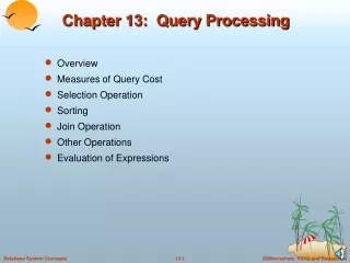
1. Chapter 13: Query Processing • Overview • Measures of Query Cost • Selection Operation • Sorting • Join Operation • Other Operations • Evaluation of Expressions

2. Basic Steps in Query Processing 1. Parsing and translation 2. Optimization 3. Evaluation

3. Query Optimization • A RA expression may have many equivalent expressions • Optimization: Amongst all equivalent expressions, choose the one with cheapest evaluation plan. • Cost is estimated using statistical information from the database catalog • e.g. number of tuples in each relation, size of tuples, etc. • Annotated RA expression specifying detailed evaluation strategy is called an evaluation-plan. • E.g., can use an index on balance to find accounts with balance < 2500, • or can perform complete relation scan and discard accounts with balance  2500

4. Measures of Query Cost • Cost is generally measured as total elapsed time for answering query • Many factors contribute to time cost • disk accesses, CPU, or even network communication • Typically disk access is the predominant cost, and is also relatively easy to estimate. Measured by taking into account • Number of seeks * average-seek-cost • Number of blocks read * average-block-read-cost • Number of blocks written * average-block-write-cost • Cost to write a block is greater than cost to read a block • data is read back after being written to ensure that the write was successful

5. Measures of Query Cost (Cont.) • For simplicity we just use number of block transfers from disk as the cost measure • We ignore the difference in cost between sequential and random I/O for simplicity • We also ignore CPU costs for simplicity. Real systems take CPU cost also into account • Costs depends on the size of the buffer in main memory • Having more memory reduces need for disk access • Amount of real memory available to buffer depends on other concurrent OS processes, and hard to determine ahead of actual execution • We often use worst case estimates, assuming only the minimum amount of memory needed for the operation is available • We do not include cost to writing output to disk.

6. Selection Operation: linear search • Algorithm A1 (linear search). Scan each file block and test all records to see whether they satisfy the selection condition. • Cost estimate (number of disk blocks scanned) = br • br denotes number of blocks containing records from relation r • If selection is on a key attribute, cost = (br /2) • stop on finding record (first or last?) • Linear search can be applied regardless of • selection condition or • ordering of records in the file, or • availability of indices

7. Selection Operation: binary search • A2 (binary search). Applicable if selection is a comparison on the attribute on which file is ordered. • Assume that the blocks of a relation are stored contiguously • Cost estimate (number of disk blocks to be scanned): • log2(br) — cost of locating the first tuple by a binary search on the blocks • Plus number of blocks containing records that satisfy selection condition

8. Selections Using Indices • Index scan – search algorithms that use an index • selection condition must be on search-key of index. • A3 (primary index on candidate key, equality). Retrieve a single record that satisfies the corresponding equality condition • Cost = HTi+ 1 • A4 (primary index on nonkey, equality) Retrieve multiple records. • Records will be on consecutive blocks • Cost = HTi+ number of blocks containing retrieved records • A5 (equality on search-key of secondary index). • Retrieve a single record if the search-key is a candidate key • Cost = HTi+ 1 • Retrieve multiple records if search-key is not a candidate key • each record may be on a different block • one block access for each retrieved record • Cost = HTi+ number of records retrieved • Can be more expensive than a linear scan.

9. Implementation of Complex Selections • Conjunction: 1 2. . . n(r) • A8 Use appropriate composite (multiple-key) index if available! • A9 Use best index and test other conditions on tuple after fetching it into memory buffer. • A10 (conjunctive selection by intersection of identifiers). • Requires indices with record pointers. • Use corresponding index for each condition, and take intersection of all the obtained sets of record pointers. • Then fetch records from file • If some conditions do not have appropriate indices, apply test in memory. • These methods are not mutually exclusive.

10. Algorithms for Complex Selections • Disjunction:1 2 . . . n(r). (disjunctive selection by union of identifiers). • Applicable if all conditions have available indices. • Otherwise use linear scan. • Use corresponding index for each condition, and take union of all the obtained sets of record pointers. • Then fetch records from file • Negation: (r) • Use linear scan on file • If very few records satisfy , and an index is applicable to  • Find satisfying records using index and fetch from file

11. Sorting • We may build an index on the relation, and then use the index to read the relation in sorted order. May lead to one disk block access for each tuple. • For relations that fit in memory, techniques like quicksort can be used. For relations that don’t fit in memory, external sort-merge is a good choice.

12. External Sort-Merge • Create sortedruns. (a) Read M blocks of relation into memory (b) Sort the in-memory blocks (c) Write sorted data to run Ri; We obtain N sorted runs • Merge the runs (N-way merge). We assume (for now) that M is the memory size (in pages).N < M. • Use N blocks of memory to buffer input runs, and 1 block to buffer output. Read the first block of each run into its buffer page • repeat • Select the first record (in sort order) among all buffer pages • Write the record to the output buffer. If the output buffer is full write it to disk. • Delete the record from its input buffer page.If the buffer page becomes empty then read the next block (if any) of the run into the buffer. • until all input buffer pages are empty: M is the memory size (in pages)

13. External Sort-Merge (Cont.) • If i M, several merge passes are required. • In each pass, contiguous groups of M - 1 runs are merged. • A pass reduces the number of runs by a factor of M -1, and creates runs longer by the same factor. • E.g. If M=11, and there are 90 runs, one pass reduces the number of runs to 9, each 10 times the size of the initial runs • Repeated passes are performed till all runs have been merged into one.

14. Example: External Sorting Using Sort-Merge

15. External Merge Sort (Cont.) • Cost analysis: • Total number of merge passes required: logM–1(br/M). • Disk accesses for initial run creation as well as in each pass is 2br • for final pass, we don’t count write cost • we ignore final write cost for all operations since the output of an operation may be sent to the parent operation without being written to disk Thus total number of disk accesses for external sorting: br ( 2 logM–1(br / M) + 1)

16. Join Operation • Several different algorithms to implement joins • Nested-loop join • Block nested-loop join • Indexed nested-loop join • Merge-join • Hash-join • Choice based on cost estimate • Examples use the following information • Number of records of customer: 10,000 depositor: 5000 • Number of blocks of customer: 400 depositor: 100

17. Nested-Loop Join • To compute the theta join rsfor each tuple tr in r do begin for each tuple tsin s do begintest pair (tr,ts) tosee if they satisfy the join condition  if they do, add tr• tsto the result.endend • r is called the outerrelation and s the inner relation of the join. • Requires no indices and can be used with any kind of join condition. • Expensive since it examines every pair of tuples in the two relations.

18. Nested-Loop Join (Cont.) • In the worst case, if there is enough memory only to hold one block of each relation, the estimated cost is nr bs + brdisk accesses. • If the smaller relation fits entirely in memory, use that as the inner relation. Reduces cost to br + bsdisk accesses. • Assuming worst case memory availability cost estimate is • 5000  400 + 100 = 2,000,100 disk accesses with depositor as outer relation, and • 1000  100 + 400 = 1,000,400 disk accesses with customer as the outer relation. • If smaller relation (depositor) fits entirely in memory, the cost estimate will be 500 disk accesses. • Block nested-loops algorithm (next slide) is preferable.

19. Block Nested-Loop Join • Variant of nested-loop join in which every block of inner relation is paired with every block of outer relation. for each block Brofr do beginfor each block Bsof s do begin for each tuple trin Br do begin for each tuple tsin Bsdo beginCheck if (tr,ts) satisfy the join condition if they do, add tr• tsto the result.end end end end

20. Block Nested-Loop Join (Cont.) • Worst case estimate: br bs + br block accesses. • Each block in the inner relation s is read once for each block in the outer relation (instead of once for each tuple in the outer relation • Best case: br+ bsblock accesses. • Various Improvements to nested loop and block nested loop algorithms: ….

21. Indexed Nested-Loop Join • Index lookups can replace file scans if • join is an equi-join or natural join and • an index is available on the inner relation’s join attribute • Can construct an index just to compute a join. • For each tuple trin the outer relation r, use the index to look up tuples in s that satisfy the join condition with tuple tr. • Worst case: buffer has space for only one page of r, and, for each tuple in r, we perform an index lookup on s. • Cost of the join: br + nr c • Where c is the cost of traversing index and fetching all matching s tuples for one tuple or r • c can be estimated as cost of a single selection on s using the join condition. • If indices are available on join attributes of both r and s,use the relation with fewer tuples as the outer relation.

22. Example of Nested-Loop Join Costs • Compute depositor customer, with depositor as the outer relation. • Let customer have a primary B+-tree index on the join attribute customer-name, which contains 20 entries in each index node. • Since customer has 10,000 tuples, the height of the tree is 4, and one more access is needed to find the actual data • depositor has 5000 tuples • Cost of block nested loops join • 400*100 + 100 = 40,100 disk accesses assuming worst case memory (may be significantly less with more memory) • Cost of indexed nested loops join • 100 + 5000 * 5 = 25,100 disk accesses. • CPU cost likely to be less than that for block nested loops join

23. Merge-Join 1. First sort both relations on their join attribute (if not already sorted on the join attributes). 2. Join step is similar to the merge stage of the sort-merge algorithm. Main difference is handling of duplicate values in join attribute — every pair with same value on join attribute must be matched.

24. Merge-Join (Cont.) • Can be used only for equi-joins and natural joins • Each block needs to be read only once (assuming all tuples for any given value of the join attributes fit in memory • Thus number of block accesses for merge-join is br + bs + the cost of sorting if relations are unsorted. • hybrid merge-join: If one relation is sorted, and the other has a secondary B+-tree index on the join attribute • Merge the sorted relation with the leaf entries of the B+-tree . • Sort the result on the addresses of the unsorted relation’s tuples • Scan the unsorted relation in physical address order and merge with previous result, to replace addresses by the actual tuples • Sequential scan more efficient than random lookup

25. Hash-Join • Applicable for equi-joins and natural joins. • A hash function h is used to partition tuples of both relations • h maps JoinAttrs values to {0, 1, ..., nh}, where JoinAttrs denotes the common attributes of r and s used in the natural join. • Hr0, Hr1, . . ., Hrnh denote partitions of r tuples • Each tuple tr r is put in partition Hr i where i = h(tr [JoinAttrs]). • Hs0, Hs1, . . ., Hsnh denotes partitions of s tuples • Each tuple tss is put in partition Hs i, where i = h(ts [JoinAttrs]).

26. Hash-Join (Cont.)

27. Hash-Join (Cont.) • r tuples in Hr ineed only to be compared with s tuples in Hsi Need not be compared with s tuples in any other partition,since: • an r tuple and an s tuple that satisfy the join condition will have the same value for the join attributes. • If that value is hashed to some value i, the r tuple has to be in Hriand the s tuple in Hsi.

28. Complex Joins • Join with a conjunctive condition: r 1  2...  ns • Either use nested loops/block nested loops, or • Compute the result of one of the simpler joins r is • final result comprises those tuples in the intermediate result that satisfy the remaining conditions 1 . . .  i –1 i +1 . . .  n • Join with a disjunctive condition r 1  2 ...  ns • Either use nested loops/block nested loops, or • Compute as the union of the records in individual joins r  is: (r 1s)  (r 2s)  . . .  (r ns)

29. Other Operations • Duplicate elimination can be implemented via hashing or sorting. • On sorting duplicates will come adjacent to each other, and all but one set of duplicates can be deleted. Optimization: duplicates can be deleted during run generation as well as at intermediate merge steps in external sort-merge. • Hashing is similar – duplicates will come into the same bucket. • Projection is implemented by performing projection on each tuple followed by duplicate elimination.

30. Other Operations (Cont.) • Aggregation can be implemented in a manner similar to duplicate elimination. • Sorting or hashing can be used to bring tuples in the same group together, and then the aggregate functions can be applied on each group. • Optimization: combine tuples in the same group during run generation and intermediate merges, by computing partial aggregate values. • Set operations (,  and ): can either use variant of merge-join after sorting, or variant of hash-join.

31. Other Operations (Cont.) • Outer join can be computed either as • A join followed by addition of null-padded non-participating tuples. • by modifying the join algorithms. • Modifying merge join to compute r s • In r s, non participating tuples are those in r – R(r s) • Modify merge-join to compute r s: During merging, for every tuple trfrom r that do not match any tuple in s, output tr padded with nulls. • Right outer-join and full outer-join can be computed similarly.

32. Evaluation of Expressions • Materialization: evaluate one operation at a time, starting at the lowest-level. Use intermediate results materialized into temporary relations to evaluate next-level operations. • E.g., in figure below, compute and storethen compute the store its join with customer, and finally compute the projections on customer-name.

33. Evaluation of Expressions (Cont.) • Pipelining: evaluate several operations simultaneously, passing the results of one operation on to the next. • E.g., in expression in previous slide, don’t store result of • instead, pass tuples directly to the join.. Similarly, don’t store result of join, pass tuples directly to projection. • Much cheaper than materialization: no need to store a temporary relation to disk. • Pipelining may not always be possible – e.g., sort, hash-join.