Download
1 / 28
300 likes | 607 Views
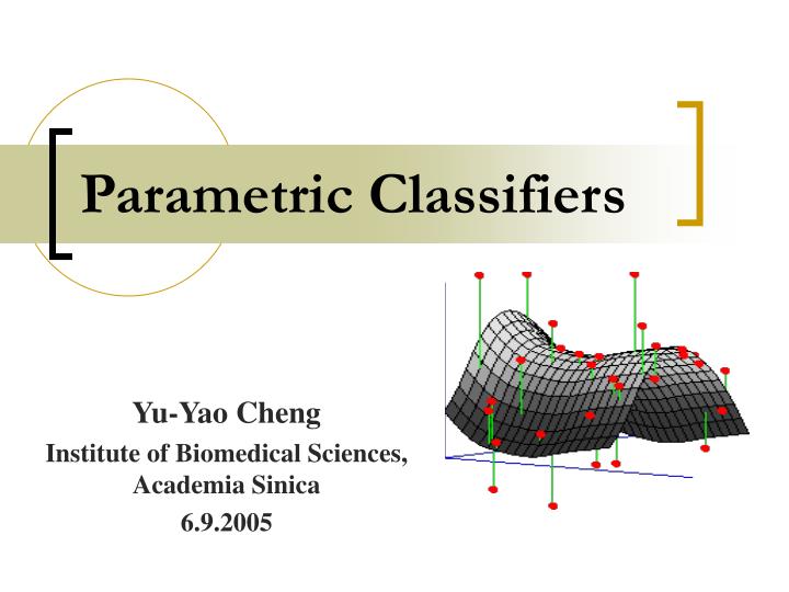
Parametric Classifiers. Yu-Yao Cheng Institute of Biomedical Sciences, Academia Sinica 6.9.2005. Contents. I. Parametric Models for Classification Decision-region boundaries Posterior probabilities Probability density functions II. Parametric Algorithms Linear regression

E N D
Parametric Classifiers Yu-Yao Cheng Institute of Biomedical Sciences, Academia Sinica 6.9.2005
Contents • I. Parametric Models for Classification • Decision-region boundaries • Posterior probabilities • Probability density functions • II. Parametric Algorithms • Linear regression • Logistic regression • Unimodal Gaussian • Example
Parametric Model for Classification Three Classification Model Types Commonly Used: • A. Decision-Region Boundaries • B. Probability Density Functions • C. Posterior Probabilities
A. Decision-Region Boundaries • To define decision regions by explicitly constructing boundaries in the input space. • To minimize the number of expected misclassifications by placing boundaries appropriately in the input space.
Decision region A. Decision-Region Boundaries (Con’t) “Ideal” but rarely happened Input #1 Class A Class B Input #2 Optimal Input #1 X Input #2
Notes:Approaches to Modeling • Parametric modeling for classification contains two stages: • Stage 1 - Parametric form is chosen based on the most natural given available information (ex: features of dataset, training/ testing time, memory req.) • Stage 2 - Parameters are tuned to fit data (learning algorithm).
A. Decision-Region Boundaries (con’t) Example of parametric form: Linear Discriminant Function (ex: Linear Regression). • To produce boundaries (hyper-plane) partitioning the input space into two half-spaces. • Parameter values specify position & orientation. • Algorithms for tuning parameters focus on finding a set of values that minimizes the number of misclassifications.
Parametric Algorithm Descriptions:Linear Regression • A multivariate linear relationship b/w var. y and var. x1, x2,…..xNcan be expressed as: X = Input variable Y = Output variable Wi = Free parameters (weights; coefficients)
Parametric Algorithm Descriptions:Linear Regression (con’t) • If the relationship is not exactly linear, then Wi’s will satisfy: Wi = Free parameters (or weights;coefficients) = Random error NEXT TASK: To find a set of parameters (Wi) that minimizes the Sum of Squared Error (SSE)!
Parametric Algorithm Descriptions: Linear Regression (con’t) “Least-Squares Minimization Procedure” • If there is n observations, the relationship b/w var. y & var. x can be expressed as: Obs. 1 Obs. 2 Obs. n
Parametric Algorithm Descriptions: Linear Regression (con’t) • Linear relationship can be expressed in matrix notation, as follows: Y = X W +
Parametric Algorithm Descriptions: Linear Regression (con’t) Y = X W + n x 1 n x (N+1) (N+1) x 1 n x 1
Parametric Algorithm Descriptions: Linear Regression (con’t) W = ?
Parametric Algorithm Descriptions: Linear Regression (con’t) Where, Xi : the i-th input pattern. di : the desired output for pattern i of the training set.
Parametric Algorithm Descriptions: Linear Regression (con’t) D = X W, W=(X’X)-1 (X’D) Xi : the i-th input pattern. di : the desired output for pattern i of the training set.
B. Posterior Probabilities • If the classification problem has m possible classes, denoted C1, C2, …, Cm. This type of model attempts to generate m posterior probabilities p(Ci|x), i=1, 2, …, m for any input vector x. • The classification is performed by identifying the input vector associated with maximal output p(Ci|x).
B. Posterior Probabilities (con’t) • Posterior probability models estimate the probability each point in the input space corresponds to each class. • Since the outputs are probability, the values are b/w 0 and 1, and sum to 1. P(CIx) Class A Class B x
B. Posterior Probabilities (con’t) Parametric technique: Logistic Regression • A sigmoid parametric form. • An effective estimation method- the sigmoid is more natural for estimating probabilities since it takes on values b/w 0 and 1, and smoothly transitions b/w the two extremes.
Parametric Algorithm Descriptions:Logistic Regression • The Logistic Regression Functions: e = natural log operator Y = outputs Xi = inputs Wi = free parameters
Parametric Algorithm Descriptions: Logistic Regression (con’t) y 1 1/2
Parametric Algorithm Descriptions: Logistic Regression (con’t) • Logistic Regression Training Flow Chart Step1: Until the stopping criteria are reached, for each pattern xk in the training set, compute the logistic output yk: where Step3
Parametric Algorithm Descriptions: Logistic Regression (con’t) Step2: Compute the gradient of the entropy error with respect to each wi due to xki:
Parametric Algorithm Descriptions: Logistic Regression (con’t) Step3: Compute the change in weights: step1 If updating weights on a per pattern basis, then update the weight; if updating once per epoch, then accumulate weight till the end of epoch.
Parametric Algorithm Descriptions: Logistic Regression (con’t) • Logistic Regression Test Flow Chart For each pattern in the test set, compute: where
Gaussian Distribution 常態分佈(normal distribution)又稱 高斯分佈(Gaussian distribution)。 德國的10馬克紙幣, 以高斯(Gauss, 1777-1855)為人像, 人像左側有一 常態分佈之P.D.F.及其圖形。
C. Probability Density Functions • The models of this type aim to construct a probability density function (PDF),p(x|C), that maps a point x in the input space to class C, reflecting its distribution in the space . • Prior probabilities,p(C), is to be estimated from the given database. • This model assigns the most probable class to an input vector x by selecting the class maximizingp(C)p(x|C).
C. Probability Density Functions (con’t) • PDF models aim at characterizing the distribution of inputs associated with each class. P(xIC) PDF Class A Class B P(xIC) X x x x x x x x x x x x x
Parametric Algorithm Descriptions: Unimodal Gaussian Bay’s Rule: Unimodal Gaussian: • Unimodal Gaussian explicitly construct the PDF, compute the prior probability P(Cj) and posterior probability P(Cj|X).