Download
1 / 185
1.86k likes | 2.01k Views
Very High Performance Cache Based Techniques for Iterative Methods. Craig C. Douglas University of Kentucky and Yale University Jonathan J. Hu Sandia National Laboratories Ulrich R ü de and Markus Kowarschik Lehrstuhl für Systemsimulation (Informatik 10) Universit ät Erlangen-Nürnberg.

E N D
Very High Performance Cache Based Techniques for Iterative Methods Craig C. Douglas University of Kentucky and Yale University Jonathan J. Hu Sandia National Laboratories Ulrich Rüde and Markus Kowarschik Lehrstuhl für Systemsimulation (Informatik 10) Universität Erlangen-Nürnberg
E-mail contacts • craig.douglas@uky.educraig.douglas@yale.edu • jhu@sandia.gov • ulrich.ruede@cs.fau.de • markus.kowarschik@cs.fau.de
Overview • Part I: Architectures and Fundamentals • Part II: Optimization Techniques for Structured Grids • Part III: Optimization Techniques for Unstructured Grids
Part I Architectures and Fundamentals
Architectures and fundamentals • Why worry about performance- an illustrative example • Fundamentals of computer architecture • CPUs, pipelines, superscalarity • Memory hierarchy • Basic efficiency guidelines • Profiling
How fast should a solver be?(just a simple check with theory) • Poisson problem can be solved by a multigrid method in < 30 operations per unknown (known since late 70’s) • More general elliptic equations may need O(100) operations per unknown • A modern CPU can do 1-6 GFLOPS • So we should be solving 10-60 million unknowns per second • Should need O(100) Mbytes of memory
How fast are solvers today? • Often no more than 10,000 to 100,000 unknowns possible before the code breaks • In a time of minutes to hours • Needing horrendous amounts of memory Even state of the art codes are often very inefficient
Compute Time in Seconds Comparison of solvers (what got me started in this business ~ '95) 10 SOR Unstructured code 1 Structured grid Multigrid 0.1 OptimalMultigrid 0.01 16384 1024 4096
Elements of CPU architecture • Modern CPUs are • Superscalar: they can execute more than one operation per clock cycle, typically: • 4 integer operations per clock cycle plus • 2 or 4 floating-point operations (multiply-add) • Pipelined: • Floating-point ops take O(10) clock cycles to complete • A set of ops can be started in each cycle • Load-store: all operations are done on data in registers, all operands must be copied to/from memory via load and store operations • Code performance heavily dependent on compiler (and manual) optimization
CPU trends • EPIC (similar to VLIW) (IA64) • Multi-threaded architectures (Alpha, Pentium4HT) • Multiple CPUs on a single chip (IBM Power 4) • Within the next decade • Billion transistor CPUs (today 200 million transistors) • Potential to build TFLOPS on a chip (e.g., SUN graphics processors) • But no way to move the data in and out sufficiently quickly!
Memory wall • Latency: time for memory to respond to a read (or write) request is too long • CPU ~ 0.5 ns (light travels 15cm in vacuum) • Memory ~ 50 ns • Bandwidth: number of bytes which can be read (written) per second • CPUs with 1 GFLOPS peak performance standard: needs 24 Gbyte/sec bandwidth • Present CPUs have peak bandwidth<10 Gbyte/sec (6.4 Itanium II) and much less in practice
Memory acceleration techniques • Interleaving (independent memory banks store consecutive cells of the address space cyclically) • Improves bandwidth • But not latency • Caches (small but fast memory) holding frequently used copies of the main memory • Improves latency and bandwidth • Usually comes with 2 or 3 levels nowadays • But only works when access to memory is local
Principles of locality • Temporal locality:an item referenced now will be referenced again soon • Spatial locality: an item referenced now indicates that neighbors will be referenced soon • Cache lines are typically 32-128 bytes with 1024 being the longest recently. Lines, not words, are moved between memory levels. Both principles are satisfied. There is an optimal line size based on the properties of the data bus and the memory subsystem designs.
Caches • Fast but small extra memory • Holding identical copies of main memory • Lower latency • Higher bandwidth • Usually several levels (2, 3, or 4) • Same principle as virtual memory • Memory requests are satisfied from • Fast cache (if it holds the appropriate copy): Cache Hit • Slow main memory (if data is not in cache): Cache Miss
Cache issues • Uniqueness and transparency of the cache • Finding the working set(what data is kept in cache) • Data consistency with main memory • Latency: time for memory to respond to a read (or write) request • Bandwidth: number of bytes that can be read (written) per second
Cache issues (cont’d) • Cache line size • Prefetching effect • False sharing (cf. associativity issues) • Replacement strategy • Least Recently Used (LRU) • Least Frequently Used (LFU) • Random • Translation lookaside buffer (TLB) • Stores virtual memory page translation entries • Has effect similar to another level of cache • TLB misses are very expensive
Effect of cache hit ratio The cache efficiency is characterized by the cache hit ratio, the effective time for a data access is The speedup is then given by
Cache effectiveness depends on the hit ratio Hit ratios of 90% and better are needed for good speedups
Cache organization • Number of cache levels • Set associativity • Physical or virtual addressing • Write-through/write-back policy • Replacement strategy (e.g., Random/LRU) • Cache line size
Cache associativity • Direct mapped (associativity = 1) • Each cache block can be stored in exactly one cache line of the cache memory • Fully associative • A cache block can be stored in any cache line • Set-associative (associativity = k) • Each cache block can be stored in one of k places in the cache Direct mapped and set-associative caches give rise to conflict misses. Direct mapped caches are faster, fully associative caches are too expensive and slow (if reasonably large). Set-associative caches are a compromise.
Typical architectures • IBM Power 3: • L1 = 64 KB, 128-way set associative (funny definition, however) • L2 = 4 MB, direct mapped, line size = 128, write back • IBM Power 4 (2 CPU/chip): • L1 = 32 KB, 2-way, line size = 128 • L2 = 1,5 MB, 8-way, line size = 128 • L3 = 32 MB, 8-way, line size = 512 • Compaq EV6 (Alpha 21264): • L1 = 64 KB, 2-way associative, line size= 32 • L2 = 4 MB (or larger), direct mapped, line size = 64 • HP PA-RISC: • PA8500, PA8600: L1 = 1.5 MB, PA8700: L1 = 2.25 MB • no L2 cache!
Typical architectures (cont’d) • AMD Athlon (from “Thunderbird” on): • L1 = 64 KB, L2 = 256 KB • Intel Pentium 4: • L1 = 8 KB, 4-way, line size = 64 • L2 = 256 KB up to 2MB, 8-way, line size = 128 • Intel Itanium: • L1 = 16 KB, 4-way • L2 = 96 KB, 6-way • L3: off-chip, size varies • Intel Itanium2 (McKinley / Madison): • L1 = 16 / 32 KB • L2 = 256 / 256 KB • L3: 1.5 or 3 / 6 MB
Basic efficiency guidelines • Choose the best algorithm • Use efficient libraries • Find good compiler options • Use suitable data layouts
Choose the best algorithm Example: Solution of linear systems arising from the discretization of a special PDE • Gaussian elimination (standard): n3/3 ops • Banded Gaussian elimination: 2n2 ops • SOR method: 10n1.5 ops • Multigrid method: 30n ops
Choose the best algorithm (cont‘d) • For n large, the multigrid method will always outperform the others, even if it is badly implemented • Frequently, however, two methods have approximately the same complexity, and then the better implemented one will win
Use efficient libraries Good libraries often outperform own software • Clever, sophisticated algorithms • Optimized for target machine • Machine-specific implementation
Sources for libraries • Vendor-independent • Commercial: NAG, IMSL, etc.; only available as binary, often optimized for specific platform • Free codes: e.g., NETLIB (LAPACK, ODEPACK, …), usually as source code, not specifically optimized • Vendor-specific; e.g., cxml for HP Alpha with highly tuned LAPACK routines
Sources for libraries (cont‘d) • Many libraries are quasi-standards • BLAS • LAPACK • etc. • Parallel libraries for supercomputers • Specialists can sometimes outperform vendor-specific libraries
Find good compiler options • Modern compilers have numerous flags to select individual optimization options • -On: successively more aggressive optimizations, n=1,...,8 • -fast: may change round-off behavior • -unroll • -arch • Etc. • Learning about your compiler is usually worth it: RTFM (which may be hundreds of pages long).
Find good compiler options (cont‘d) Hints: • Read man cc (man f77) or cc –help (or whatever causes the possible options to print) • Look up compiler options documented in www.specbench.org for specific platforms • Experiment and compare performance on your own codes
Use suitable data layout Access memory in order! In C/C++, for a 2D matrix double a[n][m]; the loops should be such that for (i...) for (j...) a[i][j]... In FORTRAN, it must be the other way round Apply loop interchange if necessary (see below)
Use suitable data layout(cont‘d) Other example: array merging Three vectors accessed together (in C/C++): double a[n],b[n],c[n]; can often be handled more efficiently by using double abc[n][3]; In FORTRAN again indices permuted
Profiling • Subroutine-level profiling • Compiler inserts timing calls at the beginning and end of each subroutine • Only suitable for coarse code analysis • Profiling overhead can be significant • E.g., prof, gprof
Profiling (cont‘d) • Tick-based profiling • OS interrupts code execution regularly • Profiling tool monitors code locations • More detailed code analysis is possible • Profiling overhead can still be significant • Profiling using hardware performance monitors • Most popular approach • Will therefore be discussed next in more detail
Profiling: hardware performance counters Dedicated CPU registers are used to count various events at runtime: • Data cache misses (for different levels) • Instruction cache misses • TLB misses • Branch mispredictions • Floating-point and/or integer operations • Load/store instructions • Etc.
Profiling tools: DCPI • DCPI = Digital Continuous Profiling Infrastructure (still supported by current owner, HP; source is even available) • Only for Alpha-based machines running Tru64 UNIX • Code execution is watched by a profiling daemon • Can only be used from outside the code • http://www.tru64unix.compaq.com/dcpi
Profiling tools: valgrind • Memory/thread debugger and cache profiler (4 tools). Part of KDE project: free. • Run usingcachegrind programNot an intrusive library, uses hardware capabilities of CPUs. • Simple to use (even for automatic testing). • Julian Seward et al • http://valgrind.kde.org
Profiling tools: PCL • PCL = Performance Counter Library • R. Berrendorf et al., FZ Juelich, Germany • Available for many platforms (Portability!) • Usable from outside and from inside the code (library calls, C, C++, Fortran, and Java interfaces) • http://www.fz-juelich.de/zam/PCL
Profiling tools: PAPI • PAPI = Performance API • Available for many platforms (Portability!) • Two interfaces: • High-level interface for simple measurements • Fully programmable low-level interface, based on thread-safe groups of hardware events (EventSets) • http://icl.cs.utk.edu/projects/papi
Profiling tools: HPCToolkit • High level portable tools for performance measurements and comparisons • Uses browser interface • PAPI should have looked like this • Make a change, check what happens on several architectures at once • http://www.hipersoft.rice.edu/hpctoolkit • Rob Fowler et al, Rice University, USA
HPCToolkit Philosophy 1 • Intuitive, top down user interface for performance analysis • Machine independent tools and GUI • Statistics to XML converters • Language independence • Need a good symbol locator at run time • Eliminate invasive instrumentation • Cross platform comparisons
HPCToolkit Philosophy 2 • Provide information needed for analysis and tuning • Multilanguage applications • Multiple metrics • Must compare metrics which are causes versus effects (examples: misses, flops, loads, mispredicts, cycles, stall cycles, etc.) • Hide getting details from user as much as possible
HPCToolkit Philosophy 3 • Eliminate manual labor from analyze, tune, run cycle • Collect multiple data automatically • Eliminate 90-10 rule • 90% of cycles in 10% of code… for a 500K line code, the hotspot is only 5,000 lines of code. How do you deal with a 5K hotspot??? • Drive the process with simple scripts
Our reference code • 2D structured multigrid code written in C • Double precision floating-point arithmetic • 5-point stencils • Red/black Gauss-Seidel smoother • Full weighting, linear interpolation • Direct solver on coarsest grid (LU, LAPACK)
Using PCL – Example 1 • Digital PWS 500au • Alpha 21164, 500 MHz, 1000 MFLOPS peak • 3 on-chip performance counters • PCL Hardware performance monitor: hpm • hpm –-events PCL_CYCLES, PCL_MFLOPS ./mg hpm: elapsed time: 5.172 s hpm: counter 0 : 2564941490 PCL_CYCLES hpm: counter 1 : 19.635955 PCL_MFLOPS