Download
1 / 101
1.03k likes | 1.24k Views
Computer Science CPSC 502 Uncertainty Probability and Bayesian Networks (Ch. 6). Outline. Uncertainty and Probability Marginal and Conditional Independence Bayesian networks. Where are we?. Representation. Reasoning Technique. Stochastic. Deterministic. Environment. Problem Type.

E N D
Computer Science CPSC 502 Uncertainty Probability and Bayesian Networks (Ch. 6)
Outline • Uncertainty and Probability • Marginal and Conditional Independence • Bayesian networks
Where are we? Representation Reasoning Technique Stochastic Deterministic • Environment Problem Type Arc Consistency Constraint Satisfaction Vars + Constraints Search Static Belief Nets Logics Variable Elimination Query Search Decision Nets Sequential STRIPS Variable Elimination Planning Search Done with Deterministic Environments Markov Processes Value Iteration
Where are we? Representation Reasoning Technique Stochastic Deterministic • Environment Problem Type Arc Consistency Constraint Satisfaction Vars + Constraints Search Static Belief Nets Logics Variable Elimination Query Search Decision Nets Sequential STRIPS Variable Elimination Planning Search Second Part of the Course Markov Processes Value Iteration
Where Are We? Representation Reasoning Technique Stochastic Deterministic • Environment Problem Type Arc Consistency Constraint Satisfaction Vars + Constraints Search Static Belief Nets Logics Variable Elimination Query Search Decision Nets Sequential STRIPS Variable Elimination Planning Search We’ll focus on Belief Nets Markov Processes Value Iteration
Two main sources of uncertainty (From Lecture 2) • Sensing Uncertainty: The agent cannot fully observe a state of interest. For example: • Right now, how many people are in this building? • What disease does this patient have? • Where is the soccer player behind me? • Effect Uncertainty: The agent cannot be certain about the effects of its actions. For example: • If I work hard, will I get an A? • Will this drug work for this patient? • Where will the ball go when I kick it?
Motivation for uncertainty • To act in the real world, we almost always have to handle uncertainty (both effect and sensing uncertainty) • Deterministic domains are an abstraction • Sometimes this abstraction enables more powerful inference • Now we don’t make this abstraction anymore • AI main focus shifted from logic to probability in the 1980s • The language of probability is very expressive and general • New representations enable efficient reasoning • We will see some of these, in particular Bayesian networks • Reasoning under uncertainty is part of the ‘new’ AI • This is not a dichotomy: framework for probability is logical! • New frontier: combine logic and probability
Probability as a measure of uncertainty/ignorance • Probability measures an agent's degree of beliefin truth of propositions about states of the world • Belief in a proposition fcan be measured in terms of a number between 0 and 1 • this is the probability of f • E.g. P(“roll of fair die came out as a 6”) = 1/6 ≈ 16.7% = 0.167 • P(f) = 0 means that f is believed to be definitely false • P(f) = 1 means f is believed to be definitely true • Using probabilities between 0 and 1 is purely a convention. .
Probability Theory and Random Variables • Probability Theory • system of logical axioms and formal operations for sound reasoning under uncertainty • Basic element: random variable X • X is a variable like the ones we have seen in CSP/Planning/Logic • but the agent can be uncertain about the value of X • As usual, the domain of a random variable X, written dom(X), is the set of values X can take • Types of variables • Boolean: e.g., Cancer (does the patient have cancer or not?) • Categorical: e.g., CancerTypecould be one of {breastCancer,lungCancer, skinMelanomas} • Numeric: e.g., Temperature (integer or real) • We will focus on Boolean and categorical variables
Possible Worlds • A possible world specifies an assignment to each random variable • Example: weather in Vancouver, represented by random variables - - • - Temperature: {hot mild cold} • - Weather: {sunny, cloudy} • There are 6 possible worlds: • w╞ f means that proposition f is true in world w • A probability measure (w) over possible worlds w is a nonnegative real number such that • (w) sums to 1 over all possible worlds w Because for sure we are in one of these worlds!
Possible Worlds • A possible world specifies an assignment to each random variable • Example: weather in Vancouver, represented by random variables - - • - Temperature: {hot mild cold} • - Weather: {sunny, cloudy} • There are 6 possible worlds: • w╞ f means that proposition f is true in world w • A probability measure (w) over possible worlds w is a nonnegative real number such that • (w) sums to 1 over all possible worlds w • The probability of proposition fis defined by: P(f)=Σ w╞ fµ(w). i.e. • sum of the probabilities of the worlds w in which f is true Because for sure we are in one of these worlds!
Example • Remember • The probability of proposition f is defined by: P(f)=Σ w╞ fµ(w) • sum of the probabilities of the worlds w in which f is true • What’s the probability of itbeing cloudy or cold? • µ(w3) + µ(w4) + µ(w5) + µ(w6) = 0.7
Joint Probability Distribution Definition (probability distribution) A probability distribution P on a random variable X is a function dom(X) [0,1] such that x P(X=x) • Joint distribution over random variables X1, …, Xn: • a probability distribution over the joint random variable <X1, …, Xn>with domain dom(X1) × … × dom(Xn) (the Cartesian product) • Think of a joint distribution over n variables as the n-dimensional table of the corresponding possible worlds • Each row corresponds to an assignment X1= x1, …, Xn= xn and its probability P(X1= x1,… ,Xn= xn) • E.g., {Weather, Temperature} example
Marginalization • P(X=x) = zdom(Z) P(X=x, Z = z) Marginalization over Z • Remember? • The probability of proposition f is defined by: P(f)=Σ w╞ fµ(w) • sum of the probabilities of the worlds w in which f is true • Given the joint distribution, we can compute distributions over subsets of the variables through marginalization: We also write this as P(X) = zdom(Z) P(X, Z = z). • Simply an application of the definition of probability measure!
Marginalization • P(X=x) = zdom(Z) P(X=x, Z = z) Marginalization over Z • Given the joint distribution, we can compute distributions over subsets of the variables through marginalization: • We also write this as P(X) = zdom(Z) P(X, Z = z). • This corresponds to summing out a dimension in the table. • Does the new table still sum to 1?
Marginalization • P(X=x) = zdom(Z) P(X=x, Z = z) Marginalization over Z • Given the joint distribution, we can compute distributions over subsets of the variables through marginalization: • We also write this as P(X) = zdom(Z) P(X, Z = z). • This corresponds to summing out a dimension in the table. • The new table still sums to 1. It must, since it’s a probability distribution!
Marginalization • P(X=x) = zdom(Z) P(X=x, Z = z) Marginalization over Z • P(Temperature=hot) = P(Weather=sunny, Temperature = hot)+ P(Weather=cloudy, Temperature = hot)= 0.10 + 0.05 = 0.15 • Given the joint distribution, we can compute distributions over subsets of the variables through marginalization: • We also write this as P(X) = zdom(Z) P(X, Z = z). • This corresponds to summing out a dimension in the table. • The new table still sums to 1. It must, since it’s a probability distribution!
Marginalization P(X=x) = z1dom(Z1),…, zndom(Zn) P(X=x, Z1 = z1, …, Zn = zn) i.e., Marginalization over Temperature and Wind • We can also marginalize over more than one variable at once
Marginalization P(X=x,Y=y) = z1dom(Z1),…, zndom(Zn) P(X=x, Y=y, Z1 = z1, …, Zn = zn) • We can also get marginals for more than one variable
Marginalization P(X=x,Y=y) = z1dom(Z1),…, zndom(Zn) P(X=x, Y=y, Z1 = z1, …, Zn = zn) • The probability of proposition f is defined by: P(f)=Σ w╞ fµ(w) • sum of the probabilities of the worlds w in which f is true • We can also get marginals for more than one variable • Still simply an application of the definition of probability measure!
Conditioning • Conditioning: revise beliefs based on new observations • Build a probabilistic model (the joint probability distribution, JPD) • Take into account all background information • Called the prior probability distribution • Denote the prior probability for proposition h as P(h) • Observe new information about the world • Call all information we received subsequently the evidencee • Integrate the two sources of information • to compute the conditional probability P(h|e) • This is also called the posterior probability of h given e.
Example for conditioning • Now, you look outside and see that it’s sunny • You are now certain that you’re in one of worlds w1, w2, or w3 • To get the conditional probability P(T|W=sunny) • renormalize µ(w1), µ(w2), µ(w3) to sum to 1 • µ(w1) + µ(w2) + µ(w3) = 0.10+0.20+0.10=0.40 • You have a prior for the joint distribution of weather and temperature
Example for conditioning • Now, you look outside and see that it’s sunny • You are now certain that you’re in one of worlds w1, w2, or w3 • To get the conditional probability P(T|W=sunny) • renormalize µ(w1), µ(w2), µ(w3) to sum to 1 • µ(w1) + µ(w2) + µ(w3) = 0.10+0.20+0.10=0.40 • You have a prior for the joint distribution of weather and temperature
Conditional Probability • Definition (conditional probability) • The conditional probability of proposition h given evidence e is • P(e): Sum of probability for all worlds in which e is true • P(he):Sum of probability for all worlds in which both h and e are true
Conditional Probability among Random Variables It expresses the conditional probability of each possible value for X given each possible value for Y P(X | Y) = P(X , Y) / P(Y) P(X | Y) = P(Temperature | Weather) = P(Temperature Weather) / P(Weather) Crucial that you can answer this question. Think about it at home and let me know if you have questions next time • Which of the following is true? • The probabilities in each row should sum to 1 • The probabilities in each column should sum to 1 • Both of the above • None of the above
Inference by Enumeration • Great, we can compute arbitrary probabilities now! • Given: • Prior joint probability distribution (JPD) on set of variables X • specific values e for the evidence variables E (subset of X) • We want to compute: • posterior joint distribution of query variables Y (a subset of X) given evidence e • Step 1: Condition to get distribution P(X|e) • Step 2: Marginalize to get distribution P(Y|e)
Inference by Enumeration: example • Given P(W,C,T) as JPD below, and evidence e : “Wind=yes” • What is the probability that it is hot? I.e., P(Temperature=hot | Wind=yes) • Step 1: condition to get distribution P(X|e)
Inference by Enumeration: example • Given P(X) as JPD below, and evidence e : “Wind=yes” • What is the probability that it is hot? I.e., P(Temperature=hot | Wind=yes) • Step 1: condition to get distribution P(X|e) • P(X|e)
Inference by Enumeration: example • Given P(X) as JPD below, and evidence e : “Wind=yes” • What is the probability that it is hot? I.e., P(Temperature=hot | Wind=yes) • Step 1: condition to get distribution P(X|e)
Inference by Enumeration: example • Given P(X) as JPD below, and evidence e : “Wind=yes” • What is the probability that it is hot? I.e., P(Temperature=hot | Wind=yes) • Step 2: marginalize to get distribution P(Y|e)
Problems of Inference by Enumeration • If we have n variables, and d is the size of the largest domain • What is the space complexity to store the joint distribution? • We need to store the probability for each possible world • There are O(dn) possible worlds, so the space complexity is O(dn) • How do we find the numbers for O(dn) entries? • Time complexity O(dn) • In the worse case, need to sum over all entries in the JPD • We will look at an alternative way to perform inference, Bayesian networks • Formalism to exploit (conditional) independence between variables • But first, let’s look at a couple more definitions
Product Rule • By definition, we know that : • We can rewrite this to • In general
Why does the chain rule help us? • We will see how, under specific circumstances (variables • independence), this rule helps gain compactness • We can represent the JPD as a product of marginal distributions • We can simplify some terms when the variables involved are independent or conditionally independent
Outline • Uncertainty and Probability • Marginal and Conditional Independence • Bayesian networks
Marginal Independence • Intuitively: if X and Y are marginally independent, then • learning that Y=y does not change your belief in X • and this is true for all values y that Y could take • For example, weather is marginally independent from the result of a dice throw
Examples for marginal independence • Intuitively (without numbers): • Boolean random variable “Canucks win the Stanley Cup this season” • Numerical random variable “Canucks’ revenue last season” ? • Are the two marginally independent?
Examples for marginal independence • Intuitively (without numbers): • Boolean random variable “Canucks win the Stanley Cup this season” • Numerical random variable “Canucks’ revenue last season” ? • Are the two marginally independent? • No! Without revenue they cannot afford to keep their best players
Exploiting marginal independence Exponentially fewer than the JPD!
Follow-up Example • We said that “Canucks win the Stanley Cup this season”and “Canucks’ revenue last season” are not marginally independent? • But they are conditionally independent given the Canucks line-up • Once we know who is playing then learning their revenue last year won’t change our belief in their chances
Conditional Independence • Intuitively: if X and Y are conditionally independent given Z, then • learning that Y=y does not change your belief in X when we already know Z=z • and this is true for all values y that Y could take and all values z that Z could take
Example for Conditional Independence Up s2 Lit l1 • Whether light l1 is lit and the position of switch s2are not marginally independent • The position of the switch determines whether there is power in the wire w0 connected to the light
Example for Conditional Independence Up s2 Power w0 Lit l1 • Whether light l1 is lit and the position of switch s2are not marginally independent • The position of the switch determines whether there is power in the wire w0 connected to the light • However, whether light l1 is lit is conditionally independent from the position of switch s2given whether there is power in wire w0 • Once we know Power w0, learning values for any other variable will not change our beliefs about light l1 • I.e., Lit l1 is independent of any other variable given Power w0
Exploiting Conditional Independence • Recall the chain rule
Belief Networks • Belief networks and their extensions are R&R systems explicitly defined to exploit independence in probabilistic reasoning
Outline • Uncertainty and Probability • Marginal and Conditional Independence • Bayesian networks
Bayesian Network Motivation Pearl recently received the very prestigious ACM Turing Award for his contributions to Artificial Intelligence! And is going to give a DLS talk on November 8! • We want a representation and reasoning system that is based on conditional (and marginal) independence • Compact yet expressive representation • Efficient reasoning procedures • Bayesian (Belief) Networks are such a representation • Named after Thomas Bayes (ca. 1702 –1761) • Term coined in 1985 by Judea Pearl (1936 – ) • Their invention changed the primary focus of AI from logic to probability! Thomas Bayes Judea Pearl
Belief (or Bayesian) networks • Def. A Belief network consists of • a directed, acyclic graph (DAG) where each node is associated with a random variable Xi • A domain for each variable Xi represented • a set of conditional probability distributions for each node Xi given its parents Pa(Xi) in the graph P (Xi | Pa(Xi)) • The parents Pa(Xi) of a variable Xiare those variables upon which Xidepends directly • A Bayesian network is a compact representation of the JDP for a set of variables (X1, …,Xn) P(X1, …,Xn) = ∏ni= 1 P (Xi | Pa(Xi))
How to build a Bayesian network • Define a total order over the random variables: (X1, …,Xn) • If we apply the chain rule, we have P(X1, …,Xn) = ∏ni= 1 P(Xi | X1, … ,Xi-1) • For each Xi, , select as parents in the Belief network a minimal set of its predecessors Pa (Xi) such that • P(Xi | X1, … ,Xi-1) = P (Xi | Pa (Xi)) • Putting it all together, in a Belief network • P(X1, …,Xn) = ∏ni= 1 P (Xi | Pa(Xi)) Predecessors of Xi in the total order defined over the variables Xi is conditionally independent from all its other predecessors given Parents(Xi) Compact representation of the JPD - factorization over the JDP based on existing conditional independencies among the variables
Example for BN construction: Fire Diagnosis Let’s construct the Bayesian network for this • You want to diagnose whether there is a fire in a building • You receive a noisy report about whether everyone is leaving the building • If everyone is leaving, this may have been caused by a fire alarm • If there is a fire alarm, it may have been caused by a fire or by tampering • If there is a fire, there may be smoke