Luminosity Diagnostics
290 likes | 495 Views
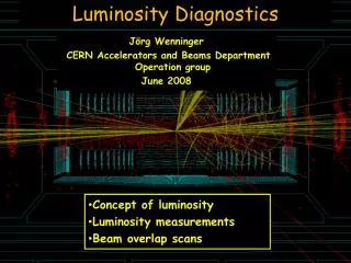
Luminosity Diagnostics. J örg Wenninger CERN Accelerators and Beams Department Operation group June 2008. Concept of luminosity Luminosity measurements Beam overlap scans. Process Cross-section.

Luminosity Diagnostics
E N D
Presentation Transcript
Luminosity Diagnostics JörgWenninger CERN Accelerators and Beams Department Operation group June 2008 • Concept of luminosity • Luminosity measurements • Beam overlap scans
Process Cross-section Consider the process where a particle encounters a target composed of a certian material – which could also be another beam. There is a certain probability that the encounter produces a certain final state composed of various particles (Higgses and SUSYs partners are very popular !). The likelyhood of the process is expressed by a CROSS-SECTION s. “Image“ : s represents the ‚area‘ over which the process occurs. • The cross-section s is expressed in units of m2. • The standard unit in nuclear & high energy physics is the barn, • 1 barn = 10-24 cm2. • Typical cross-sections for Higgs and exotic particle production are in the pico- to femtobarn range (10-36 to 10-39 cm2) .
Luminosity Definition In the case of two colliding beams, the number of collisions per unit time interval (event rate) that produce the final state of interest is proportional to the cross-section, but it also depends on how well the beams collide and how much beam there is. The luminosity L quantifies the performance (‚brillance‘) of the collider and relates the cross-section and the event rate at time t : • Units of L : m-2 s-1. • Typical luminosities: 1027 to 1034 cm-2 s-1 . • ∫L is frequently expressed in pb-1 (1036 cm-2) or fm-1 (1039 cm-2): • With ∫L = 1 pb-1 , a process with s = 1 pb yields... 1 event ! Integrating over time one obtains the integrated luminosity ∫L and the total number of events N :
Luminosity How is the luminosity related to accelerator parameters ? Intuitively the luminosity depends on: • The number of particles that collide. • The density of the particles, i.e. the beam sizes ~ particle distributions r. • The collision frequency, i.e ring size & number of bunches.
Luminosity Expression General expression of the luminosity for two bunched beams (labelled 1 and 2) : N = no. particles per bunch f = revolution frequency k = number of bunches v = speed (vector) x,y,s = coordinates x0,y,0s0 = beam offsets s = rms size c = speed of light r = density distribution of the particles, normalized to 1 Collision frequency Bunch populations Beam overlap For bunches with gaussian profiles, the distributions r can be decomposed into: with
‘Gaussian Beams’ Luminosity • The general expression for two beams with Gaussian profiles (labelled 1 and 2) colliding without crossing angle : • For beams of equal sizes this reduces to : k = number of bunches N = no. particles per bunch f = revolution frequency sx,sy = beam sizes at collision point (hor./vert.) x,y = transverse coordinates of the beam
Peak Luminosity From the expresion for beams of equal sizes One obtains the standard expression for the luminosity when the beams collide head-on (x1-x2 = y1-y2 = 0) : • The luminosity follows a gaussian profile for non-zero collision offsets. • For a separation of 1s in one plane, for example x0,1-x0,2 = sx , the reduction is exp(-1/4) ~ 0.78. Example for the LHC : k = 2808 f = 11.25 kHz N = 1.15×10¹¹ protons sx,sy = 16 mm >> L = 1.2 x 1034 cm-2 s-1
Crossing Angles x If the beams cross at an angle, the luminosity is reduced because the particles no longer traverse the entire length of the counter-rotating bunch : s f L degrades as the bunch length ‚projection‘ (ss tan(f/2)) becomes more important wrt to the transverse beam size. In all previous equations, it is assumed that the beam sizes are constant over the collision region. This is usually a good assumption, but for very strong focussing, the beam size may vary significantly over the length of the collision region. In that case numerical integration of the equation may become necessary.
L from Machine Parameters The most evident way to determine the luminosity is to compute it from machine parameters: • k, f : perfectly well known. • N : can be well known, to the level of ~ 1%. • s : more tricky! Since in general we do not have diagnostics at the collision point, it is necessary to determine the emittance and the betatron function at the IP. Difficult to obtain with much better than 5-10% accuracy. • f : measured with beam position monitors around the collision point. >> In general one does not know the luminotity to better than 5-10% from the machine parameters !
‘Van de Meer’ Scan • ISR : coasting (un-bunched) beams colliding with a crossing angle f (hor. Plane). • For a coasting beam L does not depend on the horizontal offset ! • L only depends on the vertical offset y0 and may be expressed as (Van de Meer) : x s y y0 x Gaussian profiles ∫N(y0)dy0 Area measures the beam size ! @ optimum • Just need a process that provides a signal proportional to L ! • Need excellent calibration of the scale (y0). • Beam sizes must be stable – not suited for strong beam-beam (e+e-). • In case of bunched beams scan in H & V. y0
Luminosity Measurement from s To measure the luminosity, invert the definition Now find a process that satifies the following criteria: • The process is theoretically very well established : s can be computed with the desired accuracy ! • The rate dN/dt is high (low statistical error) and can be measured with desired accuracy ! • Backgound processes contributing to dN/dt can be identified and/or their contribution can be subtracted. It is unfortunately simpler to write this down than to perform the measurement !
Bhabha Scattering For e+e- colliders, the Bhabha scattering process is normally used for luminosity measurements (g = photon): At small angle from the beam the cross-section for a detector covering the angular range (wrt beam axis) from qmin to qmax is : • Large cross-section. • Almost purely electromagnetic (QED) interaction. • Can be computed to high accuracy. LEP : < 0.05%. For high rates, aim for the smallest possible qmin
Bhabha Scattering : LEP Example • At LEP each experiments had a luminosity monitor covering the angular region of 30 to 50-100 mrad. They achieved measurements with accuracies of ~0.1%. • The LEP machine had its own detectors, based on a ‚sandwich‘ of Tungsten plates and Silicon trip detectors: • Installed at smaller angles (2-5 mrad) for faster update rates, but also more background ! • Poor(er) accuracy, calibration wrt to the monitors of the experiments. • The machine monitors were used for luminosity optimization (see later).
LEP Machine Lumi Detectors • ‚Sandwich‘ of Tungsten plates (radiation length ~3.5 mm) and Silicon detectors. • The Tungsten plates are used to induce and contain the electromagnetic particle shower. • The Si detectors consisted either of strips (S) for shower position determination or of a full plane (F) for energy measurements.
LEP L3 Experiment Detector / 1 • A Silicon track detector (SLUM) for precise impact/angle measurements. • A scintillating crytal (BGO) electro-magnetic calorimeter to measure the energy of the particle, optimized for electrons and photons.
LEP L3 Experiment Detector / 2 • The BGO detector can be ‚opened‘ to protect the sensitive BGO calorimeter from background particles during injection and ramping. • The detector was only moved to it data taking position when the beams were colliding and ‚stable‘.
The Proton Case For the case of (anti-)proton beams, it is more difficult to find processes where the threoretical cross-section is well known ! For the LHC (also TEVATRON) the processes that are potentially used : • Lepton pair production : • W/Z boson production : l = e, m X,Y = p, hadron (jet) >> theoretical errors ~ few %
The Proton Case at Small Angle An alternative for protons is to measure the cross-section at very small angles : • Measure the rates (R) for elastic and inelastic pp collisions (Rel and Rinel) [1] • Measure the dependance of the elastic rate on the momentum transfer t (~ scattering angle q) and extrapolate to t (angle) = 0 [2] dR/dt ~ dR/dq 2 1 q >> may reach ~1% This requires • Special detectors that can move very close to the beam (~ 1-4 mm !) – so called ‚Roman Pots‘ to reach angles of a few mrad. • Special optics with low divergence (and large size) beams at the collision points.
Roman Pots : TOTEM Experiment @ LHC Roman Pot tank Roman Pot Silicon tracking detectors are installed here. They can come as close a 1-4 mm to the beam. At the LHC the stored beam energy is 360 MJ !
Luminosity Optimization Very frequently the primary goal of the machine operation crews is to maximize the luminosity by achieving the best possible overlap of the beams : >> scan the beams across ech other and observe L In that case the absolute luminosity is not relevant, a relative measurement is sufficient (also true for Van de Meer Scan !) : • Any process that yields a (high) rate is OK for the luminosity measurement. • For e+e- Bhabha scatering is the optimum, for protons (ions) one can monitor anything that comes out at small angle. But watch out for systematic errors due to overlapping events (protons at high luminosity).
LHC Machine Luminosity Monitors • Machine monitors only provide relative measurements – calibration is obtained from the LHC experiments ! • The monitors are installed in an absorber for neutral particles (“TAN”). • They measure the flux of neutral particles L. • High radiation environment– as little access as possible !! : • 108 Gy / year. • Heat load > 100 W. • >1016 neutrons and charged particle per cm-2 and per year. Beam 2 Beam 1
NGAP = 6 xGAP = 1mm LHC High Luminosity Machine Detectors • Ar+N[4%] chamber. • Supposedly radiation hard. • Design optimized for high speed, but bunch by bunch measurement not fully achieved… Overlap of consecutive collisions…
LHC Low Luminosity Machine Detectors • Fast semiconductor devices. • 5·104 charges (300 mm thickness). • Radiation hard to at least 1016 n/cm-2. • Important rise in dark current at 1017 n/cm-2. • >> Used for the LHC low luminosity collision points CdTe Detectors (2 cm diameter)
Luminosity Optimization Example of luminosity optimization scans at LEP for the 4 collision points. The scans are made in each point individually. In this example one can see the luminosity for the 3 bunches in a train (a,b,c). The optimum is not the same for each bunch due to parasitic beam-beam deflections.
Beam-beam Deflections • When the beams collide, each particle senses the fields of the counter-rotating beam: the ‚beam-beam‘ force. • The beams can also be deflected collectively by the opposing beam: q1 q2 • The deflection angles may be interpolated from each side of the collision point using beam position monitors. • The total deflection angle (q1 + q2) vanishes when the offset is zero, and varies anti-symmetrically wrt to the optimimum : • >> Beam-beam deflection scan !
Luminosity Optimization by Beam-beam Deflection • Luminosity optimization by beam-beam deflection has been used extensively at SLC and at LEP2. • The analytical expression for the deflection angle is complex: • Linear near centre. • Saturation at distance of few s. • Decrease as 1/distance at large separations. • The beam parameters (size and luminosity) at the collision point can be reconstructed from the scan. • At KEKB beam-beam deflections are even used as input for collision point feedback. Deflection scan at LEP2