Download
1 / 68
770 likes | 1.31k Views
Properties of State Variables. Outline. • Asymptotic stability. • BIBO stability. • Controllability. • Observability. • Stabilizability. • Detectability • Controllable realizations. • Observable realizations. • Parallel realization. Asymptotic Stability.

E N D
Outline • Asymptotic stability. • BIBO stability. • Controllability. • Observability. • Stabilizability. • Detectability • Controllable realizations. • Observable realizations. • Parallel realization.
Asymptotic Stability A linear system is asymptotically stable if all its trajectories converge to the origin i.e. for any initial state x(k0), x(k) → 0 as k → ∞. Also called internal stability.
Asymptotic Stability Condition Theorem 8.1 A discrete-time linear system is asymptotically (Schur) stable if and only if all the eigenvalues of its state matrix are inside the unit circle.
BIBO Stability • Poles of z-transfer function inside the unit circle. • Asymptotic stability implies BIBO stability. • For a minimal system (not in general), BIBO stability implies asymptotic stability (no pole-zero cancellation).
Example 8.4 Test the BIBO stability of the system • All poles are inside the unit circle. • The system is BIBO stable.
Controllability and Observability The concepts of controllability and observability, introduced first by Kalman, play an important role in both theoretical and practical aspects of modern control. The conditions on controllability and observability essentially govern the existence of a solution to an optimal control problem. This seems to be the basic difference between optimal control theory and classical control theory. In the classical control theory, the design techniques are dominated by trial-and-error methods so that given a set of design specifications the designer at the outset does not know if any solution exists. Optimal control theory, on the other hand, has criteria for determining at the outset if the design solution exists for the system parameters and design objectives.
Controllability and Observability The condition of controllability of a system is closely related to the existence of solutions of state feedback for assigning the values of the eigenvalues of the system arbitrarily. The concept of observability relates to the condition of observing or estimating the state variables from the output variables, which are generally measurable.
Controllability Definition A system is said to be controllable if for any initial state x(k0) there exists a control sequenceu(k), k = k0 , ..., k0 +1, kf− 1, such that an arbitrary final state x(kf) can be reached in finite kf.
Controllability Condition The process is said to be completely controllable if every state variable of the process can be controlled to reach a certain objective infinite time by some unconstrained control 'u(f). Intuitively, it is simple to understand that, if any one of the state variables is independent of the control u(t), there would be no way of driving this particular state variable to a desired state in finite time by means of a control effort. Therefore, this particular state is said to be uncontrollable, and, as long as there is at least one uncontrollable state, the system is said to be not completely controllable or, simply, uncontrollable.
Uncontrollable System As a simple example of an uncontrollable system. Because the control U(t) affects only the state x1(t) the state x2(t) is uncontrollable.
Controllability Condition Theorem 8.4 A linear time-invariant system is completely controllable iff the products,Bd, i = 1,2,..., n, are all nonzero where is the ith left eigenvector of the state matrix. Furthermore, modes for which the product is zero are uncontrollable.
Controllability Rank Condition Theorem 8.5 A LTI system is completely controllable if and only if the n×m.ncontrollability matrix has rank n.
Example 8.5 Determine the controllability of the following state-equation
Solution • Controllability matrix has rank 3: controllable. • First 3 columns of matrix linearly independent: sufficient to conclude controllability. • In general, compute more columns until n linearly independent columns are obtained.
Observability A system is said to be observable if any initial state x(k0) can be estimated from the control sequence u(k), k =k0, k0+1, …, kf− 1, and the measurements y(k ), k = k0, k0+1, …, kf.
The concept of observability Essentially, a system is completely observable if every state variable of the system affects some of the outputs. In other words, it is often desirable to obtain information on the state variables from the measurements of the outputs and the inputs.
Unobservable System State diagram of a system that is not observable.
Observability Condition Theorem 8.8 A system is observable iffCviis nonzero for i = 1, 2, … , n, where viis the ith eigenvector of the state matrix. Furthermore, if the product Cviis zero then the ith mode is unobservable.
Observability Rank Test Theorem 8.9 A LTI system is completely observable iff the l.n× n observability matrix has rank n.
Example 8.10 Determine the observability of the system using two different tests. If the system is not completely observable, determine the unobservable modes.
Solution State matrix in companion form.
Rank Test • Rank = 2 • One unobservable mode.
Stabilizability & Detectability Definition 8.4 Stabilizability A system is stabilizable if all its uncontrollable modes decay to zero asymptotically. Definition 8.6 Detectability A system is detectable if all its unobservable modes decay to zero asymptotically.
Stabilizability A slightly weaker notion than controllability is that of Stabilizability. A system is determined to be stabilizable when all uncontrollable states have stable dynamics. Thus, even though some of the states cannot be controlled (as determined by the controllability test above) all the states will still remain bounded during the system's behavior
Example 8.9 Determine the controllability and stabilizability of the system Solution The system is in normal form and its input matrix has one zero row corresponding to its zero eigenvalue. Hence, the system is uncontrollable. However, the uncontrollable mode at the origin is asymptotically stable, and the system is therefore stabilizable.
Detectability A slightly weaker notion is Detectability. A system is detectable if and only if all of its unobservable modes are stable. Thus even though not all system modes are observable, the ones that are not observable do not require stabilization.
Example 8.12 Determine the observability and detectability of the system Solution The system is in normal form, and its output matrix has one zero column corresponding to its eigenvalue -2. Hence, the system is unobservable. The unobservable mode at -2, |-2| > 1, is unstable, and the system is therefore not detectable.
Realizations • Realizations give digital filter or controller implementation. • Obtained from either the z-transfer functions or the difference equation (Here: SISO transfer functions only).
Example 8.18 Obtain the controllable canonical realization of the difference equation using basic principles then show how the realization can be written by inspection from the transfer function or the difference equation
By Inspection n = 3, n − 1=2 ⇒ orders of zero matrices •The coefficients of the last row appear in the difference equation with their signs reversed. •The same coefficients appear in the denominator of the transfer function
Comments • State-space equations can be written by inspection from the difference equation or the transfer function. • Simulation diagram: shows how to implement the system with summers, delays and gains. • For an nth order system we need: n delay elements, two summers and at most 2 n + 1 gains. • Operations can be easily implemented using a microprocessor or DSP chip.
Example 8.19 Write the state-space equations in controllable canonical form for the following transfer functions
Solution (a) • Same denominator and same state equation as Example 8.18. • Numerator = (−0.05 + 0.5 z + 0 z2) output equation