Download
1 / 69
690 likes | 876 Views
BSFQ: Bin Sort Fair Queueing. Shun Y. Cheung and Corneliu S. Pencea IEEE INFOCOM 2002. Abstract. Existing packet schedulers that provide fair sharing of an output link can be divided into two classes : Sorted priority methods: excellent approximation for Weighted Fair Queueing (WFQ)

E N D
BSFQ: Bin Sort Fair Queueing Shun Y. Cheung and Corneliu S. Pencea IEEE INFOCOM 2002
Abstract • Existing packet schedulers that provide fair sharing of an output link can be divided into two classes: • Sorted priority methods: excellent approximation for Weighted Fair Queueing (WFQ) • Frame-based methods: more computationally efficient. • Bin Sort Fair Queueing (BSFQ) combines the strengths of both type of schedulers.
I. Introduction • Quality of service provisioning to flows is realized by insulatingthe flows from one another. • Fluid Fair Queueing (FFQ) • Ideal one to ensure fairness • Data of active flows are transmitted one bit at a time in a round robin fashion. • Not practical • Packets must be transmitted in their entirety. • WFQ (Weighted Fair Queueing) WF2Q (Worst-case Fair Weighted Fair Queueing) • Most accurately approximation of FFQ. • Computationally expensive
Other more efficient scheduling techniques (1)Priority-basedschemes • Packets are assigned a priority value (some function of their departure time). • Packets are transmitted in increasing order of their priority values. Fairness guarantee Some sort procedure is used to maintain a priority queue and have non-constantper packet run time complexities. • VC (Virtual Clock) • LFVC (Leap ForwardVirtual Clock) • SCFQ (Self-Clocked Fair Queueing)
(2) Frame-based schemes • Packets are transmitted in rounds. They do not use sort operations and have constantper packetprocessing time. The delay guarantee they provide have a larger bound than sorted-priority methods. • DRR (Deficit Round Robin) • URR (Uniform Round Robin)
II. Related Work • FFQ (Fluid Fair Queueing)GPS (General Processor Sharing) • Ideal • Bit-wise scheduling • Not practical • Packets must be transmitted as an atomic unit. • PFQ (Packet-by-packet Fair Queueing) • Practical • Packet-wise scheduling • To approximate FFQ • Examples • WFQ (Weighted Fair Queueing) and WF2Q (Worst-case Fair Weighted Fair Queueing)
A flow is backloggedif it has some packets in the output buffer. • A packet scheduling method is fairif the difference in the normalized service provided to any two flows that are continuously backlogged over any interval is bounded by some constant • The normalized servicewf(t1,t2) received by flow f is defined as • wf(t1, t2) is the amount of data of flow f transmitted in [t1, t2] • rf is the reserveddata rate of f.
If a scheduling discipline is fair then there is a constant ε such that |wf(t1,t2) – wg(t1,t2)|≦ ε,for any two flows f and g that are backlogged during the interval [t1,t2]. • For FFQ, |wf(t1,t2) – wg(t1,t2)| = 0. • WFQ and WF2Q approximate FFQ
WFQ and WF2Q • Compute the virtualfinish time of a packet • Transmit the packets in ascending order. • WFQ does so for every packet. • WF2Q only considers those packets that would have started receiving service. (Head-of-line) • The most accurate approximation of FFQ • Less computationally efficient
Real arrival time service time vts of previous packet • Virtual Clock (VC) method • Assign the jth packet pjf of flow f with the virtual time stamp (vts): for j > 0, where • A(pjf) = arrival time of packet pjf • ljf= length of packet pjf • vtsVC(p0f) = 0 • vtsVC(pjf) = estimated finish time of packet pjf
vts = t vts vts(p4f) δ4f vts(p3f) δjf= ljf / rf δ3f A4<vts3 vts(p2f) A3<vts2 δ2f A2>vts1 vts(p1f) δ1f t vts(p0f) A(p3f) A(p4f) A(p2f) A(p1f)
VC provides delay guarantee. • Xie and Lam showed that if the sum of the rate of all flows sharing a link does not exceedthe link capacity, the departure timeL(pjf) of packet pjfis bounded by where • lfmax is the maximumpacket length of flow f • R is the data rate of the output link. • vtsVC(pjf) = estimated finish timeL(pjf) = real finish time • VC does not providefairness guarantee.
Leap Forward Virtual Clock (LFVC) • LFVC temporarily moves oversubscribed flows into a low priorityholding area. • Only flows in the high priority area will receive service. • A flow is oversubscribed if the difference between the virtual time stamp of the current packet and the system time exceeds a certain threshold. • When all flows are oversubscribed, the system clock is advanced forward to allow some flows to be moved into high priority area.
Virtual arrival time service time vts of previous packet • Self-Clocked Fair Queueing (SCFQ) • A virtual system clockτ(t) equals to the virtual time stamp of the packet that is being serviced at time t. • The jth packet pjf of flow f is assigned with the virtual time stamp (vts):
vts vts(p5f) δ5f vts(p4f) τ4<vts4 δjf= ljf / rf δ4f vts(p3f) svt3=vts3 δ3f τ3=vts2 τ4<vts3 vts(p2f) svt2=vts2 δ2f τ2=svt1 vts(p1f) svt1=vts1 t δ1f vts(p0f) A(p2f) A(p3f) A(p4f) A(p6f) A(p1f)
Deficit Round Robin (DRR) • Packets of different flows are placed in separate queues. • Each flow is assigned a quantum size. • Each flow has a deficit counter that measures the current unused portion of the allocated bandwidth. • Packets are transmitted in rounds. • In each round, each backlogged flow is transmittedup to the sum of its quantum and deficit counter. • The unused portion of this amount is carried over to the next round as the deficit counter value.
Uniform Round Robin (URR) • Cell-based method • Space cell transmission uniformly over a round. • Example • Four flows: A, B, C, and D, each with quantum value of qA= 3, qB = qC = qD = 1. • Transmission order • For DRR: A, A, A, B, C, D • For URR: A, B, A, C, A, D
III. Bin Sort Fair Queueing • BSFQ is a frame-based method and uses virtual time stamps to determine the scheduling order. • The virtual time space is divided into equal intervals or bins. • Packets are assigned virtual time stamps and inserted into their corresponding bins. • The queueing order within a bin is FIFO.
The output buffer is organized into N bins. • Each bin is implicitly labeled with a virtual time interval and each interval has fixed length Δ. • BSFQ maintains a virtual system clockτ(t) which is equal to the left end point of the virtual time interval of the current bin at time t. • Whenever all packets in the current bin are transmitted, τ(t) is incremented by Δ. The virtual time clock in BSFQ is a non-decreasingstep function.
vts t A(p4f) A(p6f) A(p3f) A(p5f) A(p2f) A(p1f) δjf= ljf / rf Δ= 5 (Fig.3) vts(p6) δ6f A6<vts5 bin3 vts(p5) δ5f vts(p4f) bin2 δ4 vts(p3f) δ3f vts(p2f) A5<vts4 bin1 δ2f A4<vts3 vts(p1f) bin0 δ1f vts(p0f)
Virtual time stamp for pjf • The indexijfof the bin used to store pjf • If ijf= 0 then pjf is stored in the current bin. • If ijf <N then pjf is stored in the ijf –th bin. • If ijf> N then pjf is discarded.
For BSFQ τ1A = 0 +9000/3000 = 3τ2A = 3 +9000/3000 = 6τ3A = 6 +9000/3000 = 9… … τ1B = 0 +9000/1000 = 9τ2B = 9 +9000/1000 = 18τ3B = 18 +9000/1000 = 27… • Example • Flow A and B • rA = 3000 bps and rB = 1000 bps • All packets are 9000 bits in length. • A large number of packets from both flows arrive at the switch simultaneously at t = 0.
For BSFQ τ1A = 0 +9000/3000 = 3τ2A = 3 +9000/3000 = 6τ3A = 6 +9000/3000 = 9… τ1B = 0 +9000/1000 = 9τ2B = 9 +9000/1000 = 18τ3B = 18 +9000/1000 = 27…
To accommodate non-conformant flows • those do not make reservations • Define the residual rate • Packets from non-conformant flows are assigned a time stamp using rres and then scheduled in the same manner as other conformant flows
A. Delay Guarantee • A packet scheduler is in class GR if the departure timeL(pjf) of packet pjf is bounded byfor some constant β. • GRC(pjf) for j > 0 is defined as: • GRC(p0f) = 0. (3)
The end-to-end delaydif of packet pjf that traverse a path of K nodes, each using GR scheduler, is bounded by where GRC1(pjf) = GRC(pjf) at node 1, A1(pjf) = the arrival time of pjf at the first node, βn = the constant of node n on the path δn,n+1 =propagation delay between nodes n and n+1
If flow f is a leaky bucket compliant flow with parameters (σf, ρf), then
Lemma 1 • The number of bits of data Dkadmitted into k consecutive bins is bounded by: • Proof • ???
Corollary 1 • The number of bits of data D admitted into consecutive bins labeled from [τ1, τ1+Δ) to [τ2, τ2+Δ), τ1 > τ2, is bounded by • Proof • ???
Theorem 1 • The departure timeLBSFQ(pjf) of pjf in BSFQ is bounded by • Proof • ???
τ(L(pjf))+Δ vts(pjf) Estimated finish time Δ Case 1:vst(pj-1f) τ(L(pjf)) Case 2:A(pjf) L(pjf) B. Fairness Guarantee • Let L(pjf) = departure time of packet pjf • At time t = L(pjf), BSFQ is servicing the bin with the label [τ(L(pjf)), τ(L(pjf)) +Δ). • ∴τ(L(pjf)) ≦ vts(pjf)< τ(L(pjf)) +Δ (8) v t
v vst(pj-1f) τ(L(pj-1f) τ(A(pjf)) t A(pjf) L(pj-1f) • Lemma 2 • If flow f is backlogged at time t = A(pjf), then (8a) • Proof
pk1f pk1+1f pk2f pk2+1f t2 t1 L(pk1f) L(pk1+1f) L(pk2f) L(pk2+1f) • Theorem 2 • If flows f and g are backlogged during the interval [t1, t2], then (8b) • Proof • Let {pk1f, pk1+1f, …, pk2f} denote the set of packets from flow f that depart in [t1, t2].
pk1f pk1+1f pk2f pk2+1f t2 t1 L(pk1f) L(pk1+1f) L(pk2f) L(pk2+1f) • ∵Backlogged∴A(pif) < L(pi-1f) for i = k1, k1+1, …, k2, k2+1 (9)
τ(t2) τ(L(pk2f)) τ(L(pk1f)) τ(t1) t t2 t1 L(pk1f) L(pk2f) • ∵Non-decreasing step, ∴ (9a) v
τ(L(pk2f)) • From (8) τ(L(pjf)) ≦ vts(pjf)< τ(L(pjf)) +Δ we have vts(pk2f) – Δ < τ(L(pk2f)) and τ(L(pk1f)) ≦ vts(pk1f) • Thus becomes vts(pk2f) – Δ vts(pk1f) τ(L(pk1f)) (9a) (9b)
From Lemma 2 Thus …… Summing all Thus (9b) becomes (9d)
To find upper bound • From (9) • From (9d) (9e) (Move Δ to the left) (ReplaceΣwith 9e) (10)
v vts(pk1f) τ(A(pk1f)) vts(pk1-1f) t A(pk1f) • To find a lower bound, consider two cases: (1) thus (2) thus Hint: (9x) (9y)
v τ(L(pk2+1f)) τ(t2) τ(L(pk2f)) τ(L(pk1f)) τ(t1) t τ(L(pk1-1f)) t2 L(pk1-1f) t1 L(pk1f) L(pk2f) L(pk2+1f) • (Case 1) • Since no packet departure in [t1, L(pk1f)], thus L(pk1-1f) ≦t1∴
vts(pk2+1f) • From (8) τ(L(pjf)) ≦ vts(pjf)< τ(L(pjf)) +Δ we have vts(pk1-1f) – Δ < τ(L(pk1-1f)) and τ(L(pk2+1f)) ≦ vts(pk2+1f) • Thus becomes τ(L(pk2+1f)) (10x) τ(L(pk1-1f)) (10y) vts(pk1-1f) – Δ (10a) (10b)
From Lemma 2 Thus …… Summing all Thus (10b) becomes (10z) (10d)
To find lower bound • From (9) • From (10d) (10e) (Move Δ to the left) (ReplaceΣwith 10e) (11)
v τ(L(pk2+1f)) τ(t2) τ(L(pk2f)) τ(L(pk1f)) τ(t1) t τ(A(pk1f)) t2 A(pk1f) t1 L(pk1f) L(pk2f) L(pk2+1f) • (Case 2) • Since no packet departure in [t1, L(pk1f)], thus A(pk1f) ≦t1∴
∵ (10x) ∵ (10z) ∵ (9y) (11a)
From (9) • From (11a) • We have • ∵(11) < (12) ∴we take (11) as the lower bound To find lower bound (12) (11)
From (10) (11) we have (13)
From (13), we have • Thus ( subtracting) (13)