Download

1 / 11
120 likes | 162 Views
Bayesian belief networks are compact probabilistic models that represent causal relationships among variables. Explore their power in modeling causes and effects across various domains. Learn about nodes, links, and conditional probability tables.

E N D
Bayesian Belief Network Compiled By: Raj GaurangTiwari Assistant Professor SRMGPC, Lucknow
Bayesian Belief Network • Bayesian belief networks are powerful tools for modeling causes and effects in a wide variety of domains. • They are compact networks of probabilities that capture the probabilistic relationship between variables, as well as historical information about their relationships. • These networks also offer consistent semantics for representing causes and effects
Bayesian Belief Networks A (directed acyclic) graphical model of causal relationships Represents dependency among the variables Gives a specification of joint probability distribution Y Z P • Nodes: random variables • Links: dependency • X and Y are the parents of Z, and Y is the parent of P • No dependency between Z and P • Has no loops/cycles X 3
Bayesian Belief Network • Each of the variables in the Bayesian belief network are represented by nodes. • Each node has states, or a set of probable values for each variable. Nodes are connected to show causality with an arrow indicating the direction of influence. These arrows are called edges.
Example • A belief network consists of nodes (labeled with uppercase bold letters) and their associated discrete states (in lowercase). Thus node A has states {a1, a2, ...}, which collectively are denoted simply a; node B has states {b1, b2, ...}, denoted b, and so forth. The links between nodes represent direct causal influence. For example the link from A to D represents the direct influence of A upon D. In this network, the variables at B may influence those at D, but only indirectly through their effect on C. Simple probabilities are denoted P(a) and P(b), and conditional probabilities P(c|b), P(d|a, c) and P(e|d).
Conditional probability tables • Every node also has a conditional probability table, or CPT, associated with it. • Conditional probabilities represent likelihoods based on prior information or past experience. • A conditional probability is stated mathematically as , i.e. the probability of variable X in state x given parent P1 in state p1, parent P2 in state p2, ..., and parent Pn in state pn. • That is, for each parent and each possible state of that parent, there is a row in the CPT that describes the likelihood that the child node will be in some state.
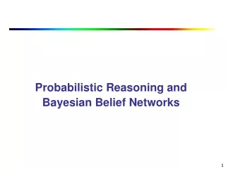
Probability Review Variables and Distributions • Let a be a discrete variable with N states: • a = { a1, a2, ..., aN } • Then P(a) is the probability distribution of a. • P(a) = {P(a1), P(a2), ... P(aN)} • Where P(a1) + ... + P(aN) = 1
Probability Review • Joint Events If a = { a1, a2, a3 } and b = { b1, b2, b3 } then P(a,b) is the joint probability distribution of a and b. • P(a,b) = {P(a1,b1), P(a1,b2), ..., P(a3,b3) } • where P(ai,bj) is the probability of event ai and bj
Probability Review • Chain Rule • We know that P( a,b) = P(a|b) P(b) • This can be expanded to three or more variables: • P(a,b,c) = P(a|b,c) P(b,c) = P(a|b,c) P(b|c) P(c) • P(a,b,c,d) = P(a|b,c,d) P(b|c,d) P(c|d) P(d) • This is known as the chain rule.
Belief Network for Fish B1: North Atlantic B2: South Atlantic A1: Winter A2: Spring A3:Summer A4:Autumn A Season B Location X Fish X1: Salmon X2: Sea Bass C Lightness C1: Light C2:Medium C3:Dark D Thickness D1: Wide D2: Thin
Example for instance the probability that the fish was caught in the summer in the north Atlantic and is a sea bass that is dark and thin: P (a3, b1, x2, c3, d2) = P (a3)P(b1)P(x2|a3, b1)P(c3|x2)P(d2|x2) = 0.25 × 0.6 × 0.4 × 0.5 × 0.4 = 0.012.