Download
1 / 4
40 likes | 281 Views
What if the population standard deviation, s , is unknown ? We could estimate it by the sample standard deviation s which is the square root of the sample variance But what becomes of the standardized mean when s estimates s ?

E N D
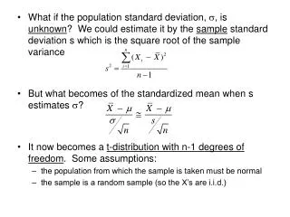
What if the population standard deviation, s, is unknown? We could estimate it by the sample standard deviation s which is the square root of the sample variance • But what becomes of the standardized mean when s estimates s? • It now becomes a t-distribution with n-1 degrees of freedom. Some assumptions: • the population from which the sample is taken must be normal • the sample is a random sample (so the X’s are i.i.d.)
Properties of t-distribution w/ n degrees of freedom (df): • symmetric around zero (mean is zero) • “bell shaped” like the normal but with a little more area in the tails • standard deviation depends upon the degrees of freedom: s.d.= Note: this exceeds 1 but as the sample size increases, s.d. approaches 1. In fact, it can be shown that as n increases to infinity, the t-distribution with n degrees of freedom approaches the standard normal distribution. As a rule of thumb, you may use the normal approximation when n is larger than 30 or so... see Table 4, last row, compared with previous rows... • Tail probabilities can be found in Table 4 in the back of the book (or you may use the TI-83: (tcdf is the function under 2nd vars...). These are denoted by ta - see Table 4... • the normal population assumption on the previous slide is not too restrictive... can you simulate with R to see this??
Now let’s look at the sampling distribution of the sample variance s2 when the X’s come from a normal population...Theorem 6.4 shows that a simple function of the sample variance has a chi-square distribution with n-1 degrees of freedom. The chi-square density is just a gamma density with alpha=(#df/2) and beta=2. Here n = n-1 = # d.f. • Properties of the chi-square distribution: • non-symmetric; P(chi-square < 0) = 0. • use the gamma(n/2, 2) distribution to see that the mean of a chi-square with n degrees of freedom is n and the variance is 2n.
The final distribution in section 6.4 is the F-distribution which arises as the quotient of two chi-squares, but we generally see it as the quotient of two sample variances where the numerator df=n1 – 1= n1and denominator df=n2 – 1= n2. • As with normal, t, and chi-square, the F-distribution is tabulated in Table 6 (and on the TI-83: Fcdf) • HW: Finish reading section 6.4 • use R to get plots of the density curves of various t, chi-square and F distributions... I’ll get you started in class today. • do # 6.20-6.26 on page 221. • do # 6.31-6.33, 6.35, 6.36 on pages 223-224.