Download
1 / 8
80 likes | 92 Views
Sections 7.1, 7.2, 7.3. Discounted cash flow analysis is a generalization of annuities with any pattern of payments and/or withdrawals. We shall assume that deposits (contributions) into, and withdrawals (returns) from, an investment occur at equally spaced times 0, 1, 2, …, n.

E N D
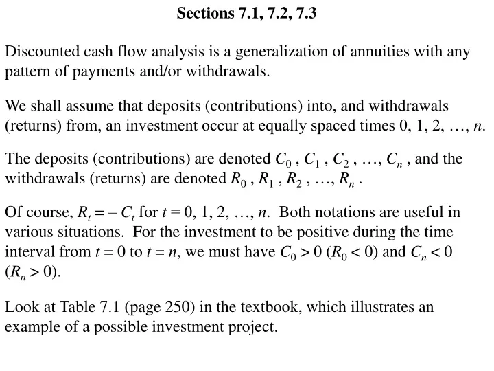
Sections 7.1, 7.2, 7.3 Discounted cash flow analysis is a generalization of annuities with any pattern of payments and/or withdrawals. We shall assume that deposits (contributions) into, and withdrawals (returns) from, an investment occur at equally spaced times 0, 1, 2, …, n. The deposits (contributions) are denoted C0 , C1 , C2 , …, Cn , and the withdrawals (returns) are denoted R0 , R1 , R2 , …, Rn . Of course, Rt = – Ct for t = 0, 1, 2, …, n. Both notations are useful in various situations. For the investment to be positive during the time interval from t = 0 to t = n, we must have C0 > 0 (R0 < 0) and Cn < 0 (Rn > 0). Look at Table 7.1 (page 250) in the textbook, which illustrates an example of a possible investment project.
Suppose that the rate of interest per period is i. Using the discounted cash flow technique, the net present value at rate i of investment returns is n t = 0 P(i) = vtRt which could be positive or negative, depending on i. For the investment project of Table 7.1 in the textbook, P(i) is positive for sufficiently small values of i but is negative for sufficiently large values of i. The value of i for which P(i) = 0 is called the yield rate (or internal rate of return); that is, the yield rate is the rate of interest at which the present value of returns from the investment is equal to the present value of contributions into the investment. Yield rates are often used to measure how favorable or unfavorable a transaction might be. From a lender’s perspective, a higher yield rate makes a transaction more favorable. From a borrower’s perspective, a lower yield rate makes a transaction more favorable.
When the yield rate is zero (0), then the investor (lender) received no return on the investment. When the yield rate is negative (but there is no practical situation where it would be less than –1), then the investor (lender) lost money on the investment. For the investment project summarized in Table 7.1 (page 250) in the textbook, verify the equation of value given in Example 7.1 (page 254) in the textbook to find the yield rate. Suppose a sum of money could either be invested in project A which pays a 10% effective rate for six years, or be invested in project B which pays an 8% effective rate for 12 years. Find the effective rate of interest necessary for the six years after project A ends so that investing in project B would be equivalent. (1.1)6(1 + i)6 = (1.08)12 0.0604 i =
In many commonly encountered financial transactions, the yield rate is unique. However, consider the yield rate in the following transaction: In exchange for receiving $230 at the end of one year, an investor pays $100 immediately and pays $132 at the end of two years. The equation of value to find the yield rate is P(i) – 100 + 230v – 132v2 = 0 100(1 + i)2 – 230(1 + i) + 132 = 0 (1 + i)2– 2.3(1 + i) + 1.32 = 0 [(1 + i) – 1.1][(1 + i) – 1.2] = 0 1 + i = 1.1 or 1 + i = 1.2 i = 10% or i = 20% Observe that P(i) > 0 only for i < 0.10 or i > 0.20 . n t = 0 In general, the equation = 0 can have multiple roots. vtRt Using Descartes’ rule of signs, it is easy to show that the yield rate will be unique when Rt 0 for t = 0, 1, 2, …, k, and Rt 0 for t = k + 1, k + 2, …, n.
n t = 0 We can rewrite the equation = 0 in the following form: vtRt C0(1 + i)n + C1(1 + i)n–1 + … + Cn–2(1 + i)2 + Cn–1(1 + i) + Cn = 0 . Suppose that i* > –1 satisfies this equation, and also suppose that C0(1 + i*) + C1 > 0 , C0(1 + i*)2 + C1(1 + i*) + C2 > 0 , C0(1 + i*)3 + C1(1 + i*)2 + C2(1 + i*) + C3 > 0 , . . . C0(1 + i*)n–2 + C1(1 + i*)n–3 + … + Cn–3(1 + i*) + Cn–2 > 0 . C0(1 + i*)n–1 + C1(1 + i*)n–2 + … + Cn–2(1 + i*) + Cn–1 > 0 . These equations imply that the investment balance is positive during the time interval from t = 0 to t = n, which is a broader condition than the condition Ct 0 for t = 0, 1, 2, …, k, and Ct 0 for t = k + 1, k + 2, …, n. By assuming that j* also satisfies the equation and that (WLOG) j* > i* , we can prove by contradiction that i* must be unique.
Since 1 + j* > 1 + i* , and all balances are positive for t = 0 to t = n–1, we must have C0(1 + j*) + C1 > C0(1 + i*) + C1 , C0(1 + j*)2 + C1(1 + j*) + C2 > C0(1 + i*)2 + C1(1 + i*) + C2 , C0(1 + j*)3 + C1(1 + j*)2 + C2(1 + j*) + C3 > C0(1 + i*)3 + C1(1 + i*)2 + C2(1 + i*) + C3 , . . . C0(1 + j*)n–1 + C1(1 + j*)n–2 + … + Cn–2(1 + j*) + Cn–1 > C0(1 + i*)n–1 + C1(1 + i*)n–2 + … + Cn–2(1 + i*) + Cn–1 . From this last equation, we find that C0(1 + j*)n + C1(1 + j*)n–1 + … + Cn–2(1 + j*)2 + Cn–1(1 + j*) + Cn > C0(1 + i*)n + C1(1 + i*)n–1 + … + Cn–2(1 + i*)2 + Cn–1(1 + i*) + Cn = 0 . This is a contradiction, since it implies that j* does not satisfy C0(1 + i)n + C1(1 + i)n–1 + … + Cn–2(1 + i)2 + Cn–1(1 + i) + Cn = 0 .
We see then that if the investment balance is positive at all points throughout the investment period, then the yield rate will be unique. However, if the investment balance becomes negative at any point, then there may not be a unique yield rate. Find the yield rate in each of the following transactions: An investor is able to borrow $1000 at 8% effective for one year and immediately invest the $1000 at 12% effective for the same year. The profit at the end of the year is $40, but there is no yield rate, since the net investment is zero. An investor pays $100 immediately and receives $1 at the end of one year. – 100 + v = 0 100(1 + i) – 1 = 0 is an equation of value, where we find i = –0.99.
An investor pays $100 immediately and pays $1 at the end of one year. – 100 –v = 0 100(1 + i) + 1 = 0 is an equation of value, where we find i = –1.01. An investor pays $100 immediately and pays $1 at the end of two years. – 100 – v2 = 0 100(1 + i)2+ 1 = 0 is an equation of value, where we find i is not a real number.