Measures of Central Tendency

1. Measures of Central Tendency U. K. BAJPAI K. V. PITAMPURA

2. Measures of Central Tendency • A measures of central of tendency may be defined as single expression of the net result of a complex group • There are two main objectives for the study • of measures of central tendency • To get one single value that represent the entire data • To facilitate comparison

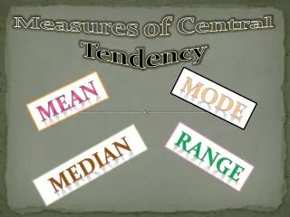
3. Measures of Central Tendency • There are three averages or measures of central tendency • Arithmetic mean • Median • Mode

4. Arithmetic Mean • The most commonly used and familiar index of central tendency for a set of raw data or a distribution is the mean • The mean is simple arithmetic average • The arithmetic mean of a set of values is their sum divided by their number

5. Merits of the Use of Mean • It is easy to understand • It is easy to calculate • It utilizes entire data in the group • It provides a good comparison • It is rigidly defined

6. Limitations • In the absence of actual data it can mislead • Abnormal difference between the highest and the lowest score would lead to fallacious conclusions • A mean sometimes gives such results as appear almost absurd. e.g. 4.3 children • Its value cannot be determined graphically

7. Calculation of Arithmetic Mean • For Ungrouped Data Mean= Sum of observations Number of observations =

8. Calculate mean for 40, 45, 50, 55, 60, 68 Mean= Sum of observations Number of observations = 40+45+50+55+60+68 6 = 318 6 Mean = 53

9. Mean of Grouped Data • The mean (or average) of observations, as we know, is the sum of the values of all the observations divided by the total number of observations. if x1, x2,. . ., xn are observations with respective frequencies f1, f2, . . ., fn, then this means observation x1 occurs f1 times, x2 occurs f2 times, and so on. • Now, the sum of the values of all the observations = f1x1 + f2x2 + . . . + fnxn, and the number of observations = f1 + f2 + . . . + fn. • We can write this in short form by using the Greek letter Σ (capital sigma) which means summation.

10. The marks obtained by 30 students of Class X of a certain school in a Mathematics paper consisting of 100 marks are presented in table below. Find the mean of the marks obtained by the students. Example

11. Solution

12. Therefore, the mean marks obtained is 59.3. In most of our real life situations, data is usually so large that to make a meaningful study it needs to be condensed as grouped data. So, we need to convert given ungrouped data into grouped data and devise some method to find its mean. Let us convert the ungrouped data of above Example into grouped data by forming class-intervals of width, say 15.

13. Now, for each class-interval, we require a point which would serve as the representative of the whole class. It is assumed that the frequency of each class interval is centred around its mid-point. So the mid-point (or class mark) of each class can be chosen to represent the observations falling in the class.

14. The mid-point of a class (or its class mark) by finding the average of its upper and lower limits. This is known as Direct Method

15. Assumed Mean Method The first step is to choose one among the xi’s as the assumed mean, and denote it by ‘a’. Also, to further reduce our calculation work, we may take ‘a’ to be that xi which lies in the centre of x1, x2, . . ., xn. So, we can choose a = 47.5 or a = 62.5. Let us choose a = 47.5.

16. Substituting the values of a, Σfidi and Σfi from Table Find the mean by taking each of xi (i.e., 17.5, 32.5, and so on) as ‘a’. You will find that the mean determined in each case is the same, i.e., 62. So, we can say that the value of the mean obtained does not depend on the choice of ‘a’.

17. Shortcut Method From the previous example the values in Column 4 are all multiples of 15. So, if we divide the values in the entire Column 4 by 15, we would get smaller numbers to multiply with fi. (Here, 15 is the class size of each class interval.)

18. So, the mean marks obtained by a student is 62.

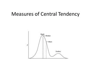
19. Median • When all the observation of a variable are arranged in either ascending or descending order the middle observation is Median. • It divides whole data into equal portion. In other words 50% observations will be smaller than the median and 50% will be larger than it.

20. Merits of Median • Like mean, median is simple to understand • Median is not affected by extreme items • Median never gives absurd or fallacious results • Median is specially useful in qualitative phenomena

21. Limitations • It is not suitable for algebraic treatment • The arrangement of the items in the ascending order or descending order becomes very tedious sometimes • It cannot be used for computing other statistical measures such as S.D or correlation

22. Calculation of Median • Un grouped data • When there is an odd number of items Median = The middle value item • When there is an even number of items Median = Sum of middle two scores 2

23. Calculate Median 7, 6, 9, 10, 4 Arrange the given data in ascending order: 4, 6, 7, 9, 10 N = 5 (odd number) Median = Middle term Median = 7 • Calculate Median 6, 9, 3, 4, 10, 5 Arrange the given data in ascending order: 3, 4, 5, 6, 9, 10 N = 6 (even number) Median= Sum of the middle two scores = 5+6 2 2 Median = 5.5

24. Grouped Data Median = l + (N/2 – F) i fm • Where, l = exact lower limit of the CI in which Median lies • F = Cumulative frequency up to the lower limit of the CI containing Median • fm = Frequency of the CI containing Median • i = Size of the class interval

25. N/2=20

26. Median = l + (N/2 – F) i fm Here, l = 50, F = 14, fm = 10, i = 10 Median = 50 + (20 – 14) * 10 10 = 50 + 6 Median = 56

27. Mode • The observation which occurs most frequently in a series is Mode

28. Merits of Mode • It can be easily located by mere inspection • It eliminates extreme variations • It is commonly understood • Mode can be determined graphically

29. Limitations • It is measure having very limited practical value • It is not capable of further mathematical treatment • It is ill-defined and indefinite and so trustworthy

30. Calculation of Mode • Ungrouped Data Mode = largest number of times that item appear • Grouped Data Mode = 3*Median – 2*Mean

31. Calculate Mode for 100, 120, 120, 100, 124, 132, 120 Mode = 120, since 120 occurs the largest number of times (3 times) • Calculate Mode for 100, 101, 110, 111, 113, 101, 113, 115 Mode = 101 & 113, since 101 and 113 occurs twice

32. For grouped data let we consider the previous problem that we solved in Mean and Median We have, Mean = 58.75 & Median = 56 Mode = 3*Median – 2*Mode = 3*56 – 2*58.75 = 168 – 117.5 Mode = 50.5

33. Thank You