Download
1 / 33
330 likes | 565 Views
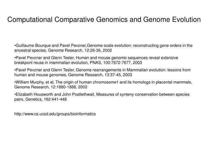
Computational Comparative Genomics and Genome Evolution. Guillaume Bourque and Pavel Pevzner,Genome-scale evolution: reconstructing gene orders in the ancestral species, Genome Research, 12:26-36, 2002

E N D
Computational Comparative Genomics and Genome Evolution • Guillaume Bourque and Pavel Pevzner,Genome-scale evolution: reconstructing gene orders in the ancestral species, Genome Research, 12:26-36, 2002 • Pavel Pevzner and Glenn Tesler, Human and mouse genomic sequences reveal extensive breakpont reuse in mammalian evolution, PNAS, 100:7672-7677, 2003 • Pavel Pevzner and Glenn Tesler, Genome rearrangements in Mammalian evolution: lessons from human and mouse genomes, Genome Research, 13:37-45, 2003 • William Murphy, et al, The origin of human chromosome1 and its homologs in placental mammals, Genome Research, 12:1880-1888, 2002 • Elizabeth Housworth and John Postlethwait, Measures of synteny conservation between species pairs, Genetics, 162:441-448 • http://www.cs.ucsd.edu/groups/bioinformatics
Why are comparative maps important? • Understanding chromosome organization and evolution • Reconstruction of ancient vertebrate chromosomes • Prediction of gene location in related species • (Comparative positional candidate approach)
Mammalian Genomes O’Brien, et al, 1999, Science 286
An Ordered Comparative Map of the Cattle and Human Genomes: Harris A. Lewin, Ph.D., Mark Band, Ph.D. Department of Animal Sciences University of Illinois at Urbana-Champaign http://cagst.animal.uiuc.edu http://www.life.uiuc.edu/biotech/
Genes that are closely linked in one species tend • to be closely linked in other species. • Genes that are loosely linked in one species tend • to be unlinked in other species. • Closely related species have accumulated fewer • rearrangements and have many long conserved segments. • Distantly related species have accumulated many • rearrangements and have many short conserved segments Nadeau and Sankoff, 1998
COMPARATIVE MAPPING METHODS Womack and Kata
Cattle and Mouse on Human Comparative Map HSA7 HSA13 Disrupted Synteny Conserved Synteny J.E.Womack et al.
BTA Prediction of Map Location HSA1p 16 2 3
COMPASS Comparative Mapping by Annotation and Sequence Similarity • Sequence similarity search (BLAST) of human Unigene database with candidate sequence • Identify human ortholog marker • Identify map position of the ortholog marker • Place the candidate sequence on human-(cattle or pig) synteny map
365 344 293 269 54 24 103 340 309 HSA5-609 404 405 537 435 HSA17 BTA16 BTA17 BTA18 BTA19 BTA20 cR5000 cR3000 cR5000 cR5000 cR3000 cR5000 cR3000 cR3000 cR3000 cR5000 0 SC4MOL CLECSF1 BM3517 MMD 0 0 0 0 671 MYOG 662 LCP2 EST0147 ATP2B4 GLG1 632 DOCK2 NPY2R 431 EST1024 AA908013 CLTCL2 SMN1 URB48 356 IDVGA31 EST1065 CA4 AF026954 BM1225 EST1409 EST1466 SCYA8 FMOD BTF3 ILSTS21 60 KIAA0727 EST0804 ILSTS85 BM6430 CDK5R1 EDNRA EST0397 EVI2B RM310 60 60 60 60 EST0605 684 HUJ614 BMS2220 NF1 C4BPB TGLA126 EST1469 CRYBA1 BM1348 0 490 EST1430 APRT INRA193 ITGA2 EST1578 R02283 EST1464 615 344 BM713 EST0004A 120 EST1050 EST0008 ADCY7 TP53 IL2 0 PAFAH1B1 EST1289 561 BM121 ATP2A3 CHRNE FGF2 SLC2A4 BM1311 ACADVL 120 120 NNT ARRB2 SLC6A2 OARFCB48 PLI INRA121 PEDF 60 TGLA53 180 BM9138 373 ILSTS14 KATNB1 SLC1A3 574 PMBP HAUT14 EPHX1 0 EST1546 723 ATP6DV 0 ETH185 BMS431 406 HSD11B2 711 EST1875 EST1302 EST0428 411 CDH3 SRP9 645 PPID* BM7109 BMS1120 180 NDP52 EST0591 240 U08018 216 EST0823 U20085 EST1042 120 OARFCB193 747 RGS7 CAPN4 THRA SELE EST0822 EST1399 116 CDH6 RPL19 611 PSA IDVGA40 PPP1R1B 60 SELL IGFBP4 ZFP36 EST0548 60 HSA5 CNP BLVRB CCNG1** PYY MIA IDVGA49 300 PSMC5 CD79A PLOD URB2 57 IDVGA47 ISG15 PAFAH1B3 GNB1 MAP2C IDVGA55 ELA1 180 BM8125 VASP TNFRSF12 PLAUR 16 APOE SDR1 427 EST2351* EST1354 120 PECAM1 360 0 269 BAX 120 MSF TBCD PTGS2 642 EST0339* 697 L04188 EST1095 CD36L1 PDE6G 485 EST0101 KCNH1 405 LCAT* 240 HUJ625 HSA6-133 COX6A1** P4HB NCF2 420 RGS16 HSA19 BM719 KRT8 DDX9 180 PLA2G1B HSA16 EST1013 CRYBB3 URB59 ADRBK2 EST0181 426 EST1517 87 EST1612 480 300 BM1233 TK1 LIF MTMR3 624 28 KIAA0106 PIK4CA 240 AANAT ICT1 HSA1 GRB2 HSA12 H3F3B 540 HSA4 HSA22 BMC1013 KCNJ2 600 EST0327 Band et al, 2000 PRKCA
BTA16 642 208.39 641.79 cR3000 cR5000 0 671 MYOG ATP2B4 FMOD EST0804 639.37 BM6430 EST0397 60 684 HUJ614 C4BPB BM1348 0 BM121 248.24 BM1311 635.71 248.34 60 TGLA53 635.11 EPHX1 723 635.1 711 EST1875 SRP9 634.49 256.94 120 747 RGS7 SELE 611 SELL IDVGA49 PLOD 57 ISG15 GNB1 264.84 ELA1 180 TNFRSF12 630.355 16 • AW462330 • (cattle EST) stSG1823 SDR1 630.345 629.89 MSF PTGS2 642 EST0339* 697 EST1095 KCNH1 240 HUJ625 NCF2 RGS16 BM719 DDX9 EST1013 EST0181 626.2 300 624 624.93 KIAA0106 624.92 HSA1 623.64 318.09 624
208.39 Cattle BAC clone • 3’End 191.6 Cattle BAC clone • 5’End 187.6 248.34 Cattle EST 186.3 256.94 176.6 318.09 HAS 1 (Mb) BTA 16 (cR)
Comparative Mapping Summary(1/00) • No. translocations: 41 • 15 cattle chromosomes with genes from only one human chromosome • 4 homologs completely conserved: BTA12-HSA13 BTA19-HSA17 BTA24-HSA18 BTAX-HSAX all have internal rearrangements
Comparative Mapping Summary(1/00) • No. conserved segments (2 or more genes): 105 • putative conserved segments (1 gene) 28 • new segments(BTA 20, BTA11, BTA25, BTA21) 4 • Centromere repositioning except possibly BTA9 and BTA23 (HSA6)
ACCURACY OF COMPASS • 333 random genes with GeneMap ‘98 map locations (GB4 panel) • correct COMPASS predictions (single assignment) 254 (76.2%) • inconsistent COMPASS predictions 19 • 7 defined new conserved segments • 8 consistent with cytogenetic mapping (GB4 mapping errors) • 15 singletons, most likely paralogs • 2 predictions by COMPASS 60 • one of 2 predictions correct 58 (97%) • Overall accuracy of COMPASS (312/333) 93.7%
HSA11 BTA15 cR5000 cR3000 319 EST0527 0 BR3510 FDX1 60 SDHD APOA1 NCAM1 PAFAH1B2 BTA29 ORP150 EST1471 120 cR5000 cR3000 JAB1 ILSTS19 0 NUCB2 EST1057 410 HSPA10 59 0 SPON1 ILSTS89 ADM OPCML 442 60 RM40 EST0614 HBB 228 X53061 RRM1 KIAA0769 36 EST0011 TRPC2 271 60 AHNAK 229 IDVGA32 ROM1 UCP3 253 114 CTSF 0 KCNA4 SIPA1 238 116 ILSTS61 BMC6004 FSHB EST0214 8 116 NAP1L4 0 RCN1 263 S68957 ILSTS81 CD44 ILSTS27 RM4 60 BM848 EXT2 F2 EST1093 C1NH LDPL 219 GAT
HSA14 HSA15 BTA10 BTA21 cR5000 cR3000 CSSM38 0 cR5000 cR3000 DDT* 295 0 IGF1R SLC24A1 335 220 HEL5 BM1237 60 AF003927 MFGE8 60 RLBP1 245 EST1037 309 PACE ILSTS94 MMP14* HSA14q11 ETH131 120 RASGRP1 111 TGLA4 BCL2A1 266 HSPCA SNAP23 120 142 UWCA4 EBP42 EST1072 ILSTS103 PPIB EST0061 EST1082 EST1435 213 EST1801 TPM1 ADAM10 KIAA0631 180 CCNB2 ARPP-19 CYP19 GALK2 EST0418 157 257 ETFA KIAA0256 INRA71 EST0843 TGLA337 0 118 AF045022 MIG2 KIAAO377 145 HIF1A GRP58 CHGA EST1550 240 EST1317 240 ILSTS54 IDVGA39 RBBP1 PI HSA11/412 NRGN** L22095 EST1368 EST1299 60 IDVGA30 WARS BMS1561 X7372 DLK1 277 EST0169 AKT1 BMS2641 300 EST1491 HE1 FOS CSSM46 LTBP2 219 L27869 AF013068.1 146 BP31 B2M Figure 2. Comparative maps for cattle chromosomes 10 and 21 with human chromosomes 14 and 15. Coverage of the human chromosomes are 46% and 56% for HSA14 and 15 respectively.
HSA1p BTA COMPASS 16 2 3
BTA29 BTA29 cR5000 cR5000 cR3000 cR3000 299 AW484109 (235cR) 9B20F7 (247cR) 16A10C7 (255cR) 7A10F6 (41cR) 9A20C11 (23cR) 10A20H12 (299cR) AW315055 (315cR) 2035 (65cR) 7A10B8 (67cR) ILSTS019 ILSTS019 0 0 315 EST1057 EST1057 65 67 ILSTS89 ILSTS89 9B10G7 (418cR) OPCML OPCML 418 443 60 60 RM40 RM40 443 EST0614 EST0614 X53061 X53061 228 228 EST0011 EST0011 AHNAK AHNAK 229 229 ROM1 ROM1 253 253 CTSF CTSF 0 0 SIPA1 SIPA1 238 238 BMC6004 BMC6004 41 EST0214 EST0214 8 8 NAP1L4 NAP1L4 263 235 GAL* GAL* ILSTS81 ILSTS81 263 HSA11 HSA11
Table 2. The detailed COMPASS prediction: QUERY_ID is the NCBI gi number. HIT_START and HIT_END are the start and end of the aligned region between the query sequences and the reference genome. REF_START and REF_END are the start and end of the base pair coordinates of either the gene marker or the conserved sequence segment on the reference genome. PREDICTED_START and PREDICTED_END are the start and end of the base pair coordinates of the conserved sequence segments on the predicting genome.
Table 3. The final COMPASS prediction results: H_START and H_END are the start and end of base pair coordinates of human genome sequences matched with the query sequences. M_START and M_END are the start and end of base pair coordinates of mouse genome sequences of the conserved region between human and mouse. R_START and R_END are the start and end of base pair coordinates of rat genome sequences of the conserved region between human and rat.
Representation of a genome We consider a unichromosomal genome to be of a sequence of n genes. The genes are represented by numbers 1, 2, ..., n. The two orientations of gene i are represented by i and -i. A genome is represented as a signed permutation of the numbers 1, 2, ..., n. For example, a unichromosomal genome with n=5 genes is 5 -3 4 2 -1 A multichromosomal genome consists of n genes spread over m chromosomes. We represent it as a signed permutation of 1, 2, ..., n, with delimiters "$" or ";" inserted between the chromosomes. For example, a genome with 12 genes spread over 3 chromosomes is 7 -2 8 3 $ 5 9 -6 -1 12 $ 11 4 10 $ The order of the chromosomes and the direction of the chromosomes do not matter in the multichromosomal algorithms. Thus, we could represent this same genome by flipping the first chromosome (reverse the order of its entries and negate them) and then moving the last chromosome to the beginning: 11 4 10 $ -3 -8 2 -7 $ 5 9 -6 -1 12 $
Unichromosomal genomes: sorting by reversal • A reversal in a signed permutation is an operation that takes an interval in a permutation, reverses the order of the numbers, and changes all their signs. For example, • 5 1 3 2 -9 7 -4 6 8 • 5 1 -7 9 -2 -3 -4 6 8 • The reversal distance between two genomes is the minimum number of reversals it takes to get from one genome to the other. For a given pair of genomes, the reversal distance is unique, but there are usually many possible reversal scenarios with this distance. However, it is possible that this mathematical notion of reversal distance can underestimate the actual number of steps that occurred biologically.
Multichromosomal genomes: rearrangement operations • We treat four elementary rearrangement events in multichromosomal genomes: reversals, translocations, fusions, and fissions. • Reversal: An interval within a single chromosome may be reversed in the same fashion as a reversal acts in the unichromosomal case: • 7 -2 8 3 $ • 5 9 -6 -1 12 $ • 11 4 10 $ • 7 -2 8 3 $ • 5 9 -12 1 6 $ • 11 4 10 $ • Note: in unichromosomal mode, the genomes • 3 1 2 and -2 -1 -3 • are considered different (one reversal apart, distance=1), while in multichromosomal mode, those same genomes are considered equivalent (distance=0) because we have simply flipped an entire chromosome, which gives an equivalent genome in the multichromosomal mode.
Translocation: Two chromosomes "A B" and "C D" may be rearranged into "A D" and "C B". (The letters A, B, C, D stand for sequences of genes.) Because flipping chromosomes does not alter a genome (only its representation is altered), "A -C" and "-B D" is another possible translocation, and is the one actually done by our algorithm. (-B means to reverse the order of the genes in sequence B and negate each one.) For example, a translocation on chromosomes 1 and 3 is 7 -2 8 3 $ 5 9 -6 -1 12 $ 11 4 10 $ 7 -2 8 -4 -11 $ 5 9 -6 -1 12 $ -3 10 $ Fusion: Two chromosomes may be fused together into a single chromosome. Due to chromosome flippings, there are four distinct fusions between each pair of chromosomes. Here is one of the fusions between chromosomes 1 and 3: 7 -2 8 3 $ 5 9 -6 -1 12 $ 11 4 10 $ 7 -2 8 3 -10 -4 -11 $ 5 9 -6 -1 12 $
Most comparative mapping techniques determine the physical locations and relative order of genes in each chromosome, but do not determine which of two orientations each gene has. Current sequencing methods do provide the orientations. It turns out that the genome rearrangement problem (uni- and multichromosomal) for unsigned permutations is NP-hard, but the same problems for signed data can be done in polynomial time. Fortunately, with many genomes currently being sequenced, it is likely that many comparative maps (corresponding to unsigned permutations) will soon be replaced by sequencing data (corresponding to signed permutations). Existing data for which signs are not known may be entered into the programs without specifying the signs. The programs will find an optimal assignment of signs, if the data is not too complex, or will approximate it otherwise. For example, to turn the unsigned genome 1 2 3 4 5 into the unsigned genome 1 4 3 2 5 requires one unsigned reversal. The program determines an assignment of signs in the source and destination genomes that give a signed reversal scenario requiring this same number of steps. Here, we get 1 2 3 4 5 1 -4 -3 -2 5 which also takes one step. Note that there may be other sign assignments taking this minimum number of steps. It is possible that correctly signed data would have increased the number of steps: 1 2 3 4 5 1 -4 -3 -2 5 1 -4 3 -2 5 If the data collection method did not determine signs, it is impossible to know mathematically whether the one step or two step scenario is more biologically accurate; the mathematical problem the program solves is to find the signs giving the minimum possible distance.