Download
1 / 19
190 likes | 198 Views
Explore sun's photospheric and coronal magnetic fields, including flux transport models and non-potential coronal models. Study features, cycle variations, and applications in solar physics.

E N D
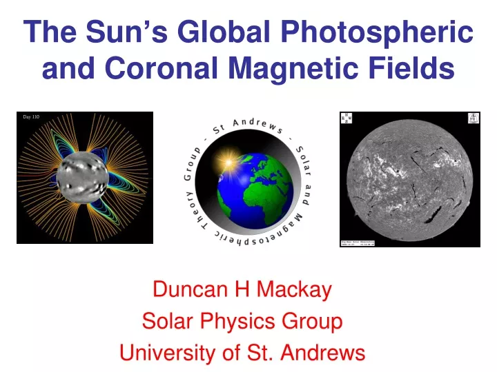
The Sun’s Global Photospheric and Coronal Magnetic Fields Duncan H Mackay Solar Physics Group University of St. Andrews
Observations • Magnetic Butterfly Diagram (Hathaway 2010) – 3.5 cycles • Sunspot Observations – 1600-pre.
Observations • Coronal Field Structure (Habbal et al. 2010) 1st August 2008 Solar Filaments (Tandberg- Open Flux (Balogh et al. 1995, Hanssen 1996, Mackay et al. 2010) Lockwood 1999, Solanki 2000)
Photospheric Magnetic Fields • Magnetic Flux Transport Models : simulate large-scale, long-time evolution of the Sun’s radial magnetic field (Wang and Sheeley 1989, van Ballegooijen et al. 1998, Schrijver (2001), Baumann et al. 2005) Flux Emergence (Observations) Surface motions: Differential Rotation Meridional Flow Surface Diffusion • Able to reproduce main features of the solar cycle: - LRSP articles : Sheeley (2005), Mackay and Yeates (2012) - problem with polar field over multiple cycles and Cycle 24.
Extensions and Outstanding Issues • Including small scale fields (Worden and Harvey 2000, Schrijver 2001) • Additional Decay terms (Schrijver et al 2002, Baumann et al. 2006) • Meridional Flow Variations : Countercell (Jiang et al. 2009), Active region inflow (DeRosa and Schrijver 2006, Jiang et al. 2010) • Polar field Issues: Loss of reversal Extra decay term(Schrijver et al 2002, Baumann et al. 2006) Cycle to cycle meridional flow variations (Wang et al 2002) Cycle to cycle variation in tilt angles (Cameron et al .2010)
Coronal Models: Potential Field • Potential Field Source Surface Models: used to extrapolate coronal magnetic fields (Scatten et al. 1969). Wide range of use: Coronal Holes: Wang and Sheeley 1990. Open Flux: Wang et al. 2000, Mackay and Lockwood 2002, Wang and Sheeley 2002. Coronal Null Points: Cook et al. 2009. Stellar Corona: Jardine et al. 2002. Properties: unique, minimum energy state • PFSS has limited use: no electric currents, free energy.
Coronal Models: Non-potential • Wide range of global non-potential models. Current Sheet Source Surface: Schatten (1971) Non-linear Force-Free Extrapolations: Optimisation method - Wiegelmann (2007) Electrodynamics method - Contopoulos et al (2011) Magnetohydrostatic Models:Neukirch (1995), Zhao et al. (2000) Ruanet al (2008) MHD Models: Riley et al. 2006, DeVore and Antiochos 2008, Downs et al . 2010, Feng et al. 2012. See Section 3 of Mackay and Yeates (2012), LRSP for details and applications. • Consider applications of non-linear force-free time evolution simulations: van Ballegooijen et al. 2000, Mackay and van Ballegooijen (2006) Yeates et al. 2008
6 month: May-Aug 1999 Non-Potential Model for the Coronal Magnetic Field • Long Term simulations (months ~ years). - Build up free magnetic energy • Two coupled components: Photosphere: Flux transport Model - includes flux emergence - accurately reproduces Br. Corona : Magnetofrictional Relaxation - quasi-static evolution - non-linear force-free states, j x B = 0 - formation/ejection of flux ropes. • Development and Application: van Ballegooijen et al 2000; Mackay and van Ballegooijen 2006a,b; Yeates et al. 2007, 2008a,b, 2009a,b.
Hemispheric Pattern of Filaments • Two types of chirality:Sinistraland Dextral. Northern Hemipshere - Dextral Southern Hemipshere – Sinistral (Martin et al. 1995, Leroy 1983,1984) • Test : Determine the chirality of filaments (6 months, 109) . Test chirality produced by model with observed chirality. Obs: Dextral Sim: Dextral
Results of Comparison • Emerge: –ve helicity bipoles ~ NH, +ve helicity bipoles ~ SH ~ dextral Shapes: observed chirality * ~ sinistral Colours: correct wrong Up to 96.9% correct • Results improve the longer the simulation is run. • Simulation describes the build-up of non-potential fields correctly. • Yeates, Mackay and van Ballegooijen 2007,2008, 2009
Full Solar Cycle Simulation – Cycle 23 • Data driven simulation 1996-2012 –accurately reproduces large-scale pattern (Yeates and Mackay 2012) • +/- 50o • dominant chirality pattern • 2007-2010 more mixed pattern • High Latitudes • Rising Phase– polar crown has dominant chirality pattern • Cycle 24 – dominant chirality. • Declining Phase – minority chirality • Clear model predictions (obs. of filament chirality carried out in rising phase.
Open Flux Models • A wide range of techniques exist for modelling the open flux. Magnitude Variation Models Spatial Distribution Models. Lockwood, Stamper & Two component models Wild (1999) Solanki et al. (2000,2002) PhotosphericBC + Coronal Model Obs. BrSim. BrPFSS CSSS Non-pot. MWO/WSO Flux Transport SS Kitt Peak Model Wang et al. 1989, 1992, 1996, 1995, 2002, 2003; Mackay et al. 2002a,b, 2006; Schrijver et al. 2002; Schussler and Baumann 1996; Riley 2007. Alternative model : Fisk and Schwadron 2001, Fisk 2005, Gilbert et al (2007).
Open Magnetic Flux • Potential field models underestimate level of open flux(Riley 2007, Schussler and Baumann 2006, Fisk and Zurbuchen 2006, Lockwood et al 2009a,b) • Three main sources of open flux (Yeates et al. 2010, JGR): - Background level (location of flux sources). - Enhancement due to: 1) inflation due to electric currents: surface motions 2) sporadic flux rope ejections: loss of equilibrium
3D Global MHD Models • Required to give self consistent description (Mikic et al. 1999,Lionello et al 2001, 2009, Downs et al. 2010) • Key Features: Resistive MHD EIT 171 Form Steady state solution. - assume initial potential field - solar wind EIT 195 Improved energy eqn: thermal cond., rad. loss, heating EIT Include: chromosphere, TR 284 SXT Most important factor in producing correct emission is heating term. (from Lionello et al. 2009)
Summary • Considered global models for solar magnetic fields • Models: input obs. data output obs. quantities • Flux transport models : Sun and Stars Produce evolving lower boundary conditions • Coronal Models : PFSS – useful but limited. Non-potential Models - based on actual observations - models build-up of coronal currents and free energy - sucessfully applied : filaments, open flux. • Global MHD models : steady state realistic energy equations form of coronal heating important for emmission.
Test 3: Coronal Mass Ejections • One mechanism is the flux rope ejection model: shearing motions, flux cancellation & loss of equilibrium (Lin et al. 2003). • Global simulations form flux ropes in time dependant manner (Yeates and Mackay 2009, Yeates et al. 2010) Comparisons: flux rope ejections and CME source locations from EIT EUV events. 4.5 months : 330 CMEs (Lasco) 98 – EIT 195 Å events correlated Outcome : +ve correlation ~ 0.49 Two classes of CMEs: ½ - gradual flux rope formation ½ - shorter time scale in AR (dynamic instability, break- out)
Photospheric Boundary Condition • Flux Transport Model • 6 month continuous simulation 6 KP synoptic maps (CR1948-1954) - Start from rotation 1948. - Evolve forward in time using flux transport effects. - Include flux emergence (119 bipoles) - Shears the surface fields ~ coronal field diverges from equilibrium. - Physical time scale.
Coupled 3D Model. • Coronal Model : Magneto-Frictional Relaxation (velocity lorentz force.) Coronal field relaxes to a non-linear force-free field, j x B = 0. Relaxation time scale ~ not physical
3D Inserting Bipoles • Bipoles are inserted as an isolated field containing either zero, +ve or –ve helicity (alpha) both in the photosphere and corona. Day 250 Day 251