Download
1 / 17
170 likes | 304 Views
Simulation. A Queuing Simulation. Example. The arrival pattern to a bank is not Poisson There are three clerks with different service rates A customer must choose which idle server to go to These conditions do not meet the restrictions of queuing models developed earlier.

E N D
Simulation A Queuing Simulation
Example • The arrival pattern to a bank is not Poisson • There are three clerks with different service rates • A customer must choose which idle server to go to • These conditions do not meet the restrictions of queuing models developed earlier
TIME BETWEEN ARRIVALS MINUTES PROB RN 1 .40 00-39 2 .30 40-69 3 .20 70-89 4 .10 90-99
SERVICE TIME FOR ANN MINUTES PROB RN 3 .10 00-09 4 .20 10-29 5 .35 30-64 6 .15 65-79 7 .10 80-89 8 .05 90-94 9 .05 95-99
SERVICE TIME FOR BOB MINUTES PROB RN 2 .05 00-04 3 .10 05-14 4 .15 15-29 5 .20 30-49 6 .20 50-69 7 .15 70-84 8 .10 85-94 9 .05 95-99
SERVICE TIME FOR CARL MINUTES PROB RN 6 .25 00-24 7 .50 25-74 8 .25 75-99
CHOICE OF SERVER ALL THREE SERVERS IDLE CHOICE PROB RN ANN 1/3 0000-3332 BOB 1/3 3333-6665 CARL 1/3 6666-9999* (* Carl’s prob. is .0001 more than 1/3) TWO SERVERS IDLE (A/B), (A/C), (B,C) CHOICE: A/BA/CB/C PROB RN Ann Ann Bob 1/2 0-4 Bob Carl Carl 1/2 5-9
ARBITRARY CHOICE OFCOLUMNS FOR SIMULATION EVENT COLUMN ARRIVALS 10 CHOICE OF SERVER 15 ANN’S SERVICE 1 BOB’S SERVICE 2 CARL’S SERVICE 3
DESIRED QUANTITIES • WQ -- the average waiting time in queue • W -- the average waiting time in system • LQ -- the average # customers in the queue • L -- the average # customers in the system • If we get estimates for Wq and W, then from Little’s Laws we can estimate: • LQ = WQ • L = W
WILL WE REACH STEADY STATE? • Average time between arrivals = 1/ = .4(1) + .3(2) + .2(3) + .1(4) = 2.0 minutes = 60/2 = 30/hr. • Ann’s average service time = 1/A = .1(3) +.2(4) + …+ .05(9) = 5.3 minutes A = 60/5.3 = 11.32/hr.
WILL WE REACH STEADY STATE? • Bob’s average service time = 1/B = .05(2) +.1(3) + …+ .05(9) = 5.5 minutes B = 60/5.5 = 10.91/hr. • Carl’s average service time = 1/C = .25(6) +.50(7) + .25(8) = 7 minutes C = 60/7 = 8.57/hr. • = 30/hr. • A + B + C = 11.32 + 10.91 + 8.57 = 30.8/hr. < A + B + C ===> Will reachSteady State!
THE SIMULATION # RN IAT AT WQ RN SERV SB RN ST SE W 1 36 1 8:01 0 4231 B 8:01 33 5 8:06 5 2 52 2 8:03 0 7 C 8:03 98 8 8:11 8 3 99 4 8:07 0 9 B 8:07 26 4 8:11 4 4 54 2 8:09 0 ------ A 8:09 88 7 8:16 7 5 96 4 8:13 0 8 C 8:13 00 6 8:19 6 6 20 1 8:14 0 ------ B 8:14 48 5 8:19 5 7 41 2 8:16 0 ------ A 8:16 11 4 8:20 4 8 31 1 8:17 2 6 C 8:19 61 7 8:26 9 9 33 1 8:18 1 ------ B 8:19 96 9 8:28 10
SIMULATION (CONT’D) # RN IAT AT WQ RN SERV SB RN ST SE W 10 07 1 8:19 1 ------ A 8:20 62 5 8:25 6 11 21 1 8:20 5 ------ A 8:25 54 5 8:30 10 12 01 1 8:21 5 ------ C 8:26 49 7 8:33 12 13 20 1 8:22 6 ------ B 8:28 84 7 8:35 13 14 18 1 8:23 7 ------ A 8:30 69 6 8:36 13 15 92 4 8:27 6 ------ C 8:33 95 8 8:41 14 16 10 1 8:28 7 ------ B 8:35 63 6 8:41 13 17 90 4 8:32 4 ------ A 8:36 31 5 8:41 9 18 66 2 8:34 7 3711 B 8:41 05 3 8:44 10
CALCULATING THE STEADY STATE QUANTITIES • The quantities we want are steady state quantities -- • The system must be allowed to settle down to steady state • Throw out the results from the first n customers • Here we use n = 8 • Average the results of the rest • Here we average the results of customers 9 -18
CALCULATIONS FOR W, Wq • Total Wait in the queue of the last 10 customers = (1+1+5+5+6+7+6+7+4+7) = 49 min. WQ 49/10 = 4.9 min. • Total Wait in the queue of the last 10 customers = (10+6+10+12+13+13+14+13+9+10) = 90 min. W 90/10 = 9.0 min.
CALCULATIONS FOR L, Lq • Little’s Laws: LQ = WQ and L = W • and W and Wq must be in the same time units • = 30/hr. = .5/min. • LQ= WQ (.5)(4.9) = 2.45 • L = W (.5)(9.0) = 4.50 • ρ = est. of system utilization 4.50 -2.45 = 2.05 • Est. of Average number of idle workers 3- 2.05 = 0.95
Review • Simulation of Queuing Models to Determine System Parameters • Check to See if Steady State Will Be Reached • Determine random number mappings • Use of pseudorandom numbers to estimate WQ and W • Ignore the results from the first few arrivals • Use Little’s Laws to get L, LQ • Average Number of Busy Workers = L - LQ