Download
1 / 23
230 likes | 324 Views
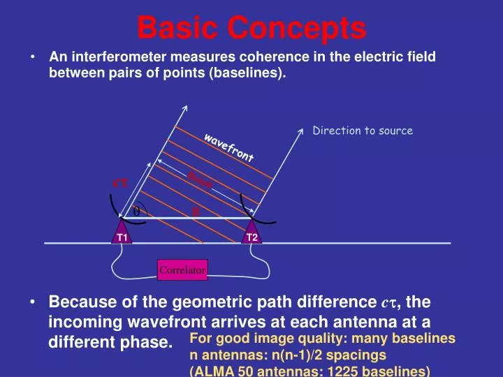
Basic Concepts. An interferometer measures coherence in the electric field between pairs of points (baselines). Direction to source. wavefront. c t. Bsin . . B. T2. T1. Correlator.

E N D
Basic Concepts • An interferometer measures coherence in the electric field between pairs of points (baselines). Direction to source wavefront ct Bsin B T2 T1 Correlator • Because of the geometric path difference ct, the incoming wavefront arrives at each antenna at a different phase. For good image quality: many baselines n antennas: n(n-1)/2 spacings (ALMA 50 antennas: 1225 baselines)
Aperture Synthesis • As the source moves across the sky (due to Earth’s rotation), the baseline vector traces part of an ellipse in the (u,v) plane. B sin = (u2 + v2)1/2 v (kl) Bsin T2 u (kl) B T1 T2 T1 • Actually we obtain data at both (u,v) and (-u,-v) simultaneously, since the two antennas are interchangeable. Ellipse completed in 12h, not 24!
Synthesis observing • Correlate signals between telescopes: visibilities • Assign the visibilities to correct position on the u-v disc • Fourier Transform the u-v plane : image
Deconvolution • There are gaps in u-v plane. Need algorithms such as CLEAN and Maximum Entropy to guess the missing information • This process is called deconvolution
visibilities dirty image clean image
Data flow “Every astronomer, including novices to aperture synthesis techniques, should be able to use ALMA” Data flow: • Data taking • Quality Assurance(QA)programme • Data reduction pipeline • Archive • User
ALMA data reduction • After every observation: • Data reduction pipeline starts • Flagging (data not fulfilling given conditions) • Calibration (antenna, baseline, atmosphere, …) bandpass, phase and amplitude, flux • Fourier transform (u-v to map) • Deconvolution • (Mosaicking, combination, ACA and main array,…) • Output: fully calibrated u-v data sets and images or cubes(x,y,freq) Archive • Pipeline part of CASA (f.k.a. aips++)
ALMA Imaging Simulations Dirty Mosaic Clean Mosaic
Dusty Disks in our Galaxy: Physics of Planet Formation Vega debris disk simulation: PdBI & ALMA Simulated PdBI image Simulated ALMA image
ALMA Resolution Simulation Contains: * 140 AU disk * inner hole (3 AU) * gap 6-8 AU * forming giant planets at: 9, 22, 46 AU with local over-densities * ALMA with 2x over-density * ALMA with 20% under-density * Each letter 4 AU wide, 35 AU high Observed with 10 km array At 140 pc, 1.3 mm Observed Model L. G. Mundy
ALMA 950 GHz simulations of dust emission from a face-on disk with a planet Simulation of 1 Jupiter Mass planet around a 0.5 Solar mass star (orbital radius 5 AU) The disk mass was set to that of the Butterfly star in Taurus Integration time 8 hours; 10 km baselines; 30 degrees phase noise (Wolf & D’Angelo 2005)
Imaging Protoplanetary Disks • Protoplanetary disk at 140pc, with Jupiter mass planet at 5AU • ALMA simulation • 428GHz, bandwidth 8GHz • total integration time: 4h • max. baseline: 10km • Contrast reduced at higher frequency as optical depth increases • Will push ALMA to its limits Wolf, Gueth, Henning, & Kley 2002, ApJ 566, L97
SMA 850 mm of Massive Star Formation in Cepheus A-East SMA 850 mm dust continuumVLA 3.6 cm free-free 1” = 725 AU 2 GHz • Massive stars forming regions are at large distances need high resolution • Clusters of forming protostars and copious hot core line emission • Chemical differentiation gives insight to physical processes ALMA will routinely achieve resolutions of better than 0.1” Brogan et al., in prep.
Orion at 650 GHz (band 9) : A Spectral Line Forest LSB USB Schilke et al. (2000)
ALMA: A Unique probe of Distant Galaxies Galaxies z < 1.5 Galaxies z > 1.5
Gravitational lensing by a cluster of galaxies submillimeter optical (simulations by A. Blain)
ALMA into the Epoch of Reionization Band 3 at z=6.4 Spectral simulation of J1148+5251 at z=6.4 • Detect dust emission in 1sec (5s) at 250 GHz • Detect multiple lines, molecules per band => detailed astrochemistry • Image dust and gas at sub-kpc resolution – gas dynamics! CO map at 0”.15 resolution in 1.5 hours CO HCO+ HCN CCH 96.1 93.2 4 GHz BW Atomic line diagnostics [C II] emission in 60sec (10σ) at 256 GHz [O I] 63 µm at 641 GHz [O I] 145 µm at 277 GHz [O III] 88 µm at 457 GHz [N II] 122 µm at 332 GHz [N II] 205 µm at 197 GHz HD 112 µm at 361 GHz
Why do we need all those telescopes? Mosaicing and Precision Imaging • SMA ~1.3 mm observations • Primary beam ~1’ • Resolution ~3” 3.0’ ALMA 1.3mm PB ALMA 0.85mm PB CFHT 1.5’ Petitpas et al. 2006, in prep.
ALMA Mosaicing Simulation Spitzer GLIMPSE 5.8 mm image • Aips++/CASA simulation of ALMA with 50 antennas in the compact configuration (< 100 m) • 100 GHz 7 x 7 pointing mosaic • +/- 2hrs
Similar effect to adding both total power from 12m and ACA need to fill in 15m gap in ALMA compact config. + 24m SD 50 antenna + Single Dish ALMA Clean results Model Clean Mosaic + 12m SD