Download
1 / 9
90 likes | 239 Views
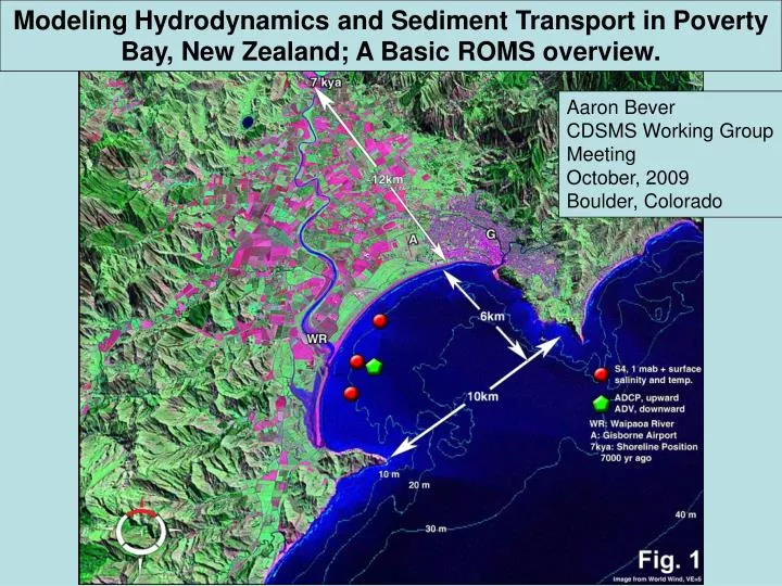
Modeling Hydrodynamics and Sediment Transport in Poverty Bay, New Zealand; A Basic ROMS overview. Aaron Bever CDSMS Working Group Meeting October, 2009 Boulder, Colorado. Regional Ocean Modeling System: ROMS. 3D hydrodynamic and “sediment transport” numerical model

E N D
Modeling Hydrodynamics and Sediment Transport in Poverty Bay, New Zealand; A Basic ROMS overview. Aaron Bever CDSMS Working Group Meeting October, 2009 Boulder, Colorado
Regional Ocean Modeling System: ROMS • 3D hydrodynamic and “sediment transport” numerical model • Fortran 90 with C preprocessing, thousands and thousands of lines • Solves Reynolds-averaged equations • Many different turbulence closure schemes • Choice of horizontal and vertical advection schemes • Serial, OMP, MPI implementation based on settings when compiled • Curvilinear horizontal and stretched terrain following vertical grids • IO based on netcdf files • Different “modules” included based on compiling parameters • Sediment, suspended load, bedload, biology, point sources, etc. • Sediment requires basic input characteristics
Poverty Bay Forcing – Somewhat different “modules” • Bathymetry was created using high resolution multibeam from within Poverty Bay, and shelf bathy provided by Scott Stephens (NIWA). 7 kya bathymetry was from Wolinsky et al. (in review). • Open boundaries used gradient conditions, and Chapman and Flather for free surface and 2D momentum, respectively. • Tides were included based on the OSU global tidal model. • Freshwaterwas hourly observations, with sediment discharge based on the rating curve of Hicks et al. (2000) (Fig. 1AB). • Meteorologywas based on observations; hourly winds from the Gisborne airport (Fig. 1C), with other variables monthly means. • Multiplefluvial sediment classes were used (table 1), representing the average grain size of the Waipaoa discharge and a coarser floc. • Time-varying 2D waves for the modern and 7kya geometries were modeled by the SWAN model, using the winds from the Gisborne airport and open boundary conditions from the WW3 global model.
Forcing – Hourly water and sediment discharge, winds Monthly means: Air temp and pressure, relative humidity, cloud cover
SWAN Waves WW3 B.C.
Other potential features • Biology: phytoplankton growth, nutrient uptake, burial in seabed, etc. • Sea ice: ??? • Data assimilation • Carbonates: ???