Chapter 5 Discrete Probability Distributions

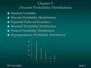
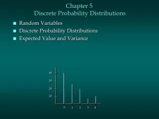
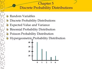
.40 .30 .20 .10 0 1 2 3 4 Chapter 5 Discrete Probability Distributions • Random Variables • Discrete Probability Distributions • Expected Value and Variance • Binomial Distribution • Poisson Distribution

5.1 Random Variables A random variable is a numerical description of the outcome of an experiment. A discrete random variable may assume either a finite number of values or an infinite sequence of values. A continuous random variable may assume any numerical value in an interval or collection of intervals.

Example: JSL Appliances • Discrete random variable with a finite number of values Let x = number of TVs sold at the store in one day, where x can take on 5 values (0, 1, 2, 3, 4)

Example: JSL Appliances • Discrete random variable with an infinite sequence of values Let x = number of customers arriving in one day, where x can take on the values 0, 1, 2, . . . We can count the customers arriving, but there is no finite upper limit on the number that might arrive.

Random Variables Type Question Random Variable x Family size x = Number of dependents reported on tax return Discrete Continuous x = Distance in miles from home to the store site Distance from home to store Own dog or cat Discrete x = 1 if own no pet; = 2 if own dog(s) only; = 3 if own cat(s) only; = 4 if own dog(s) and cat(s)

5.2 Discrete Probability Distributions The probability distribution for a random variable describes how probabilities are distributed over the values of the random variable. We can describe a discrete probability distribution with a table, graph, or equation.

Discrete Probability Distributions The probability distribution is defined by a probability function, denoted by f(x), which provides the probability for each value of the random variable. The required conditions for a discrete probability function are: f(x) > 0 f(x) = 1

Discrete Probability Distributions • Using past data on TV sales, … • a tabular representation of the probability distribution for TV sales was developed. Number Units Soldof Days 0 80 1 50 2 40 3 10 4 20 200 xf(x) 0 .40 1 .25 2 .20 3 .05 4 .10 1.00 80/200

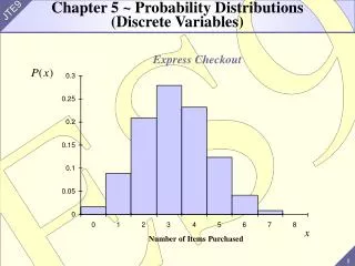
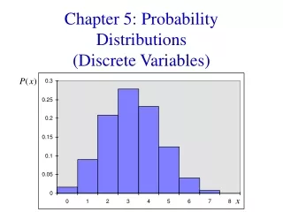
.50 .40 .30 .20 .10 Discrete Probability Distributions • Graphical Representation of Probability Distribution Probability 0 1 2 3 4 Values of Random Variable x (TV sales)

Discrete Uniform Probability Distribution The discrete uniform probability distribution is the simplest example of a discrete probability distribution given by a formula. The discrete uniform probability function is f(x) = 1/n the values of the random variable are equally likely where: n = the number of values the random variable may assume

E(x) =  = xf(x) Var(x) =  2 = (x - )2f(x) 5.2 Expected Value and Variance The expected value, or mean, of a random variable is a measure of its central location. The variance summarizes the variability in the values of a random variable. The standard deviation,, is defined as the positive square root of the variance.

Expected Value and Variance • Expected Value xf(x)xf(x) 0 .40 .00 1 .25 .25 2 .20 .40 3 .05 .15 4 .10 .40 E(x) = 1.20 expected number of TVs sold in a day

Expected Value and Variance • Variance and Standard Deviation x (x - )2 f(x) (x - )2f(x) x - -1.2 -0.2 0.8 1.8 2.8 1.44 0.04 0.64 3.24 7.84 0 1 2 3 4 .40 .25 .20 .05 .10 .576 .010 .128 .162 .784 TVs squared Variance of daily sales =s 2 = 1.660 Standard deviation of daily sales = 1.2884 TVs

End of Chapter 5

Chapter 5 Discrete Probability Distributions