Download
1 / 7
190 likes | 1.08k Views
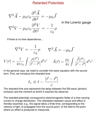
Retarded Potentials. in the Lorentz gauge. If there is no time dependence…. In the general case, we need to consider the wave equation with the source term. First, we introduce the retarded time:

E N D
Retarded Potentials in the Lorentz gauge If there is no time dependence… In the general case, we need to consider the wave equation with the source term. First, we introduce the retarded time: The retarded time and represents the delay between the EM wave (photon) emission and the moment at which it reaches the observer. The retarded potentials correspond to electromagnetic fields of a time-varying current or charge distribution. The retardation between cause and effect is thereby essential; e.g., the signal takes a finite time, corresponding to the velocity of light, to propagate from the source point of the field to the point where an effect is produced or measured.
Retarded potentials Consider a thought experiment in which a charge q appears at position r0 at time t=t1, persists for a while, and then disappears at time t2. What is the electric field generated by such a charge? otherwise (no currents)
We can now appreciate the essential difference between time-dependent electromagnetism and the action at a distance laws of Coulomb and Biot & Savart. In the latter theories, the field-lines act rather like rigid wires attached to charges (or circulating around currents). If the charges (or currents) move then so do the field-lines, leading inevitably to unphysical action at a distance type behavior. In the time-dependent theory, charges act rather like water sprinklers: i.e., they spray out the Coulomb field in all directions at the speed of light. Similarly, current carrying wires throw out magnetic field loops at the speed of light. If we move a charge (or current) then field-lines emitted beforehand are not affected, so the field at a distant charge (or current) only responds to the change in position after a time delay sufficient for the field to propagate between the two charges (or currents) at the speed of light. Liénard–Wiechert potentials Liénard-Wiechert potentials describe the classical electromagnetic effect of a moving electric point charge in terms of a vector potential and a scalar potential. Built directly from Maxwell's equations, these potentials describe the complete, relativistically correct, time-varying electromagnetic field for a point charge in arbitrary motion, but are not corrected for quantum-mechanical effects. Electromagnetic radiation in the form of waves can be obtained from these potentials. These expressions were developed in part by Alfred-Marie Liénard in 1898 and independently by Emil Wiechert in 1900. We assume that a point charge q is moving on a specified trajectory: The retarded time is given by the condition retarded position of the charge vector from the retarded position of the charge to the field point r
Only one retarded point contributes to the potentials at any given moment (charged particles cannot move with velocity of light). The difficulty is that is not the charge of the particle
Note that this has nothing to do with special relativity (Lorentz contraction). Indeed, L is the length of the moving particle and its rest length is not at issue. The argument follows that of the Doppler effect. Since the current density is Liénard–Wiechert potentials
Example: potentials of a point charge moving with constant velocity After squaring both sides and solving for tr, we obtain
The EM fields of a moving point charge When calculating derivatives one has to remember that the retarded time depends on r and t. This complicates algebra significantly. For instance where is the acceleration of the particle at the retarded time. After some algebra (Griffiths), one obtains: Griffiths (10.52) • The magnetic field of a point charge is always perpendicular to the electric field and to the vector from the retarded point. • Both fields depend both on velocity and acceleration of a moving charge!