Download

1 / 10
100 likes | 185 Views
Sampling Distributions. The Design. Consider taking 10 draws from a Uniform distribution on (0,1). [That is, randomly drawing a number between 0 and 1]. One can show that if a random variable X has such a distribution, then E(X) =.5 and Var(X) =1/12. The Design, Continued.

E N D
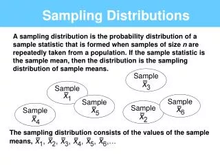
Sampling Distributions Econ 472
The Design • Consider taking 10 draws from a Uniform distribution on (0,1). [That is, randomly drawing a number between 0 and 1]. One can show that if a random variable X has such a distribution, then E(X) =.5 and Var(X) =1/12. Econ 472
The Design, Continued • Let x1, x2, , x10 denote this collection of 10 draws. • Consider two different rules for using this data to estimate E(X) = x: • and Econ 472
The Design, Continued • Both of these estimators are unbiased, since • (The fact that our first estimator is unbiased was proven in class). Econ 472
The Design, Continued • To obtain the sampling distribution of both estimators, we first obtain 5,000 different sets of 10 draws from this uniform distribution. • For each set of 10 draws, we calculate both estimates. • We summarize the 5,000 estimates from each estimator in the following histograms: Econ 472
Results for Sample Mean • As you can see, the sample mean is an unbiased estimator of the population mean x, as the sampling distribution is centered around E(X) = .5. Econ 472
Results for Second Estimator • Again, this is an unbiased estimator of x. • However, it is slightly less efficient than the sample mean, (i.e., it has a larger variance). • This becomes a little more clear when plotting the sampling distributions on the same graph: Econ 472