Download
1 / 13
130 likes | 450 Views
6.3 Segmented Least Squares. Segmented Least Squares. Least squares. Foundational problem in statistic and numerical analysis. Given n points in the plane: (x 1 , y 1 ), (x 2 , y 2 ) , . . . , (x n , y n ). Find a line y = ax + b that minimizes the sum of the squared error:

E N D
Segmented Least Squares • Least squares. • Foundational problem in statistic and numerical analysis. • Given n points in the plane: (x1, y1), (x2, y2) , . . . , (xn, yn). • Find a line y = ax + b that minimizes the sum of the squared error: • Solution. Calculus min error is achieved when y x
Segmented Least Squares • Segmented least squares. • Points lie roughly on a sequence of several line segments. • Given n points in the plane (x1, y1), (x2, y2) , . . . , (xn, yn) with • x1 < x2 < ... < xn, find a sequence of lines that minimizes f(x). • Q. What's a reasonable choice for f(x) to balance accuracy and parsimony? goodness of fit number of lines y x
Segmented Least Squares • Segmented least squares. • Points lie roughly on a sequence of several line segments. • Given n points in the plane (x1, y1), (x2, y2) , . . . , (xn, yn) with • x1 < x2 < ... < xn, find a sequence of lines that minimizes: • the sum of the sums of the squared errors E in each segment • the number of lines L • Tradeoff function: E + c L, for some constant c > 0. y x
Dynamic Programming: Multiway Choice • Notation. • OPT(j) = minimum cost for points p1, pi+1 , . . . , pj. • e(i, j) = minimum sum of squares for points pi, pi+1 , . . . , pj. • To compute OPT(j): • Last segment uses points pi, pi+1 , . . . , pj for some i. • Cost = e(i, j) + c + OPT(i-1).
Segmented Least Squares: Algorithm • Running time. O(n3). • Bottleneck = computing e(i, j) for O(n2) pairs, O(n) per pair using previous formula. INPUT: n, p1,…,pN , c Segmented-Least-Squares() { M[0] = 0 for j = 1 to n for i = 1 to j compute the least square error eij for the segment pi,…, pj for j = 1 to n M[j] = min 1 i j (eij + c + M[i-1]) return M[n] } can be improved to O(n2) by pre-computing various statistics
Knapsack Problem • Knapsack problem. • Given n objects and a "knapsack." • Item i weighs wi > 0 kilograms and has value vi > 0. • Knapsack has capacity of W kilograms. • Goal: fill knapsack so as to maximize total value. • Ex: { 3, 4 } has value 40. • Greedy: repeatedly add item with maximum ratio vi / wi. • Ex: { 5, 2, 1 } achieves only value = 35 greedy not optimal. Item Value Weight 1 1 1 2 6 2 W = 11 3 18 5 4 22 6 5 28 7
Dynamic Programming: False Start • Def. OPT(i) = max profit subset of items 1, …, i. • Case 1: OPT does not select item i. • OPT selects best of { 1, 2, …, i-1 } • Case 2: OPT selects item i. • accepting item i does not immediately imply that we will have to reject other items • without knowing what other items were selected before i, we don't even know if we have enough room for i • Conclusion. Need more sub-problems!
Dynamic Programming: Adding a New Variable • Def. OPT(i, w) = max profit subset of items 1, …, i with weight limit w. • Case 1: OPT does not select item i. • OPT selects best of { 1, 2, …, i-1 } using weight limit w • Case 2: OPT selects item i. • new weight limit = w – wi • OPT selects best of { 1, 2, …, i–1 } using this new weight limit
Knapsack Problem: Bottom-Up • Knapsack. Fill up an n-by-W array. Input: n, w1,…,wN, v1,…,vN for w = 0 to W M[0, w] = 0 for i = 1 to n for w = 1 to W if (wi > w) M[i, w] = M[i-1, w] else M[i, w] = max {M[i-1, w], vi + M[i-1, w-wi ]} return M[n, W]
0 1 2 3 4 5 6 7 8 9 10 11 0 0 0 0 0 0 0 0 0 0 0 0 { 1 } 0 1 1 1 1 1 1 1 1 1 1 1 { 1, 2 } 0 1 6 7 7 7 7 7 7 7 7 7 { 1, 2, 3 } 0 1 6 7 7 18 19 24 25 25 25 25 { 1, 2, 3, 4 } 0 1 6 7 7 18 22 24 28 29 29 40 { 1, 2, 3, 4, 5 } 0 1 6 7 7 18 22 28 29 34 34 40 Item Value Weight 1 1 1 2 6 2 3 18 5 4 22 6 5 28 7 Knapsack Algorithm W + 1 n + 1 OPT: { 4, 3 } value = 22 + 18 = 40 W = 11
Knapsack Problem: Running Time • Running time. (n W). • Not polynomial in input size! • "Pseudo-polynomial." • Decision version of Knapsack is NP-complete. [Chapter 8] • Knapsack approximation algorithm. There exists a polynomial algorithm that produces a feasible solution that has value within 0.01% of optimum. [Section 11.8]