Download
1 / 24
260 likes | 451 Views
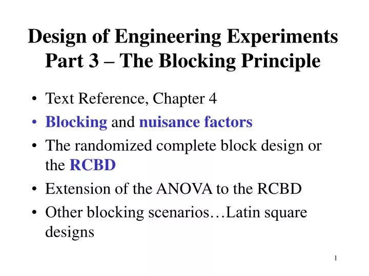
Design of Engineering Experiments Part 3 – The Blocking Principle. Text Reference, Chapter 4 Blocking and nuisance factors The randomized complete block design or the RCBD Extension of the ANOVA to the RCBD Other blocking scenarios…Latin square designs. The Blocking Principle.

E N D
Design of Engineering ExperimentsPart 3 – The Blocking Principle • Text Reference, Chapter 4 • Blocking and nuisance factors • The randomized complete block design or the RCBD • Extension of the ANOVA to the RCBD • Other blocking scenarios…Latin square designs
The Blocking Principle • Blocking is a technique for dealing with nuisancefactors • A nuisance factor is a factor that probably has some effect on the response, but it’s of no interest to the experimenter…however, the variability it transmits to the response needs to be minimized • Typical nuisance factors include batches of raw material, operators, pieces of test equipment, time (shifts, days, etc.), different experimental units • Many industrial experiments involve blocking (or should) • Failure to block is a common flaw in designing an experiment (consequences?)
The Blocking Principle • If the nuisance variable is known and controllable, we use blocking • If the nuisance factor is known and uncontrollable, sometimes we can use the analysis of covariance (see Chapter 15) to remove the effect of the nuisance factor from the analysis • If the nuisance factor is unknown and uncontrollable (a “lurking” variable), we hope that randomization balances out its impact across the experiment • Sometimes several sources of variability are combined in a block, so the block becomes an aggregate variable • Blocking is a technique to systematically eliminate the effect of nuisance factors
The Hardness Testing Example • Text reference, pg 119 • We wish to determine whether 4 different tips produce different (mean) hardness reading on a Rockwell hardness tester • Gauge & measurement systems capability studies are frequent areas for applying DOX • Assignment of the tips to an experimental unit; that is, a test coupon • The test coupons are a source of nuisance variability • Alternatively, the experimenter may want to test the tips across coupons of various hardness levels • The need for blocking • Structure of a completely randomized experiment
The Hardness Testing Example • To conduct this experiment as a RCBD, assign all 4 tips to each coupon • Each coupon is called a “block”; that is, it’s a more homogenous experimental unit on which to test the tips • Variability between blocks can be large, variability within a block should be relatively small • In general, a block is a specific level of the nuisance factor • A complete replicate of the basic experiment is conducted in each block • A block represents a restriction on randomization • All runs within a block are randomized
The Hardness Testing Example • Suppose that we use b = 4 blocks: • “complete” – each block (coupon) contains all the treatments (tips) • “randomized” – runs are randomized in each block • Once again, we are interested in testing the equality of treatment means, but now we have to remove the variability associated with the nuisance factor (the blocks)
Extension of the ANOVA to the RCBD • Suppose that there are a treatments (factor levels) and b blocks • A statistical model (effects model) for the RCBD is • The relevant (fixed effects) hypotheses are
Extension of the ANOVA to the RCBD ANOVA partitioning of total variability:
Extension of the ANOVA to the RCBD The degrees of freedom for the sums of squares in are as follows: Therefore, ratios of sums of squares to their degrees of freedom result in mean squares and the ratio of the mean square for treatments to the error mean square is an F statistic that can be used to test the hypothesis of equal treatment means
ANOVA Display for the RCBD MSBlocks/MSE cannot be used as an F statistic to evaluate the equality of block means because the runs are not randomized between blocks. However, the ratio can be used to approximate the effect of blocking variable. Large ratio implies a large blocking effect and that blocking helps improving precision of comparison of treatment means. Manual computing …see Equations (4-9) – (4-12), page 124 Design-Expert analyzes the RCBD
Hardness Testing Revisited The analysis can be conducted in terms of coded data (keep it in mind when interpreting the results)
ANOVA of Hardness Testing Revisited SourceSum ofDegrees ofMeanFof VariationSquaresDFFreedomSquareValueProb > F Treatments 38.50 3 12.83 14.44 0.0009 (Type of tip) Blocks (coupons) 82.50 3 27.50Error 8.00 9 0.89 Total 129.00 15 • = 0.05, critical F0.05,3,9 = 3.86 < 14.44. Therefore, the means of the tip types are not equal, or they affect mean hardness reading. The mean square for blocks is large relative to error, so the blocks (coupons) differ significantly.
What if the experiments were completely randomized? ANOVA of Hardness Testing (Incorrect analysis – totally randomized) SourceSum ofDegrees ofMeanFof VariationSquaresDFFreedomSquareValue Type of tip 38.50 3 12.83 1.70 Error 90.50 12 7.54 Total 129.00 15 • = 0.05, critical F0.05,3,12 = 3.49 > 1.70. Therefore, the hypothesis of equal mean hardness measurements cannot be rejected – contradict to previous analysis.
Residual Analysis for the Hardness Testing Experiment • Basic residual plots indicate that normality, constant variance assumptions are satisfied • No obvious problems with randomization • Can also plot residuals versus the type of tip (residuals by factor) and versus the block • These plots provide more information about the constant variance assumption, possible outliers
Vascular Grafts (Ex. 4-1, pg. 124) There might be batch-to-batch variation, so resin is chosen as block factor RCBD
ANOVA of Vascular Graft Experiment • = 0.05, critical F0.05,9,15 = 3.29 < 8.1. Therefore, the means of the extrusion pressures are not equal, or they affect mean yield. The mean square for blocks is large relative to error, so the blocks (coupons) differ significantly.
What if the experiments were completely randomized? As P-value < 0.05, we still reject the null hypothesis and conclude that extrusion pressure significantly affect the mean yield. However, the mean square for error increases from 7.33 in the RCBD to 15.11 as the variability due to blocks is in the error term – the inflated experimental error may make it impossible to identify the important differences among the treatment means.
Residual Analysis for the Vascular Graft Experiment • Basic residual plots indicate that normality, constant variance assumptions are satisfied • No obvious problems with randomization • These plots provide more information about the constant variance assumption, possible outliers
Multiple Comparisons for the Vascular Graft Experiment – Which Treatments are Different? Treatment Means (Adjusted, If Necessary) EstimatedStandardMeanError 1-8500 92.82 1.10 2-8700 91.68 1.10 3-8900 88.92 1.10 4-9100 85.77 1.10 MeanStandard t for H0TreatmentDifferenceDFErrorCoeff=0 Prob > |t| 1 vs 2 1.13 1 1.56 0.73 0.4795 1 vs 3 3.90 1 1.56 2.50 0.0247 1 vs 4 7.05 1 1.56 4.51 0.0004 2 vs 3 2.77 1 1.56 1.77 0.0970 2 vs 4 5.92 1 1.56 3.79 0.0018 3 vs 4 3.15 1 1.56 2.02 0.0621 Center part of Fig. 4-2 Fisher LSD procedure: m1 = m2, m1 is different from all others, m2≠m3 (roughly), and m2 ≠ m4.
Other Aspects of the RCBDSee Text, Section 4-1.3, pg. 136 • The RCBD utilizes an additive model – no interaction between treatments and blocks • Treatments and/or blocks can be treated as random effects • Missing values (use approximate methods) • Sample sizing in the RCBD? The OC curve approach can be used to determine the number of blocks to run..see page 131