Download

1 / 13
170 likes | 458 Views
CHAPTER 22 MONEY DEMAND. THEORY OF MONEY DEMAND. Money demand is proportional to nominal income: M d = kPY where k is assumed stable at equilibrium conditions. Fisher on the Quantity Theory of Money: MV = PY where V = 1/k is also assumed stable.

E N D
CHAPTER 22MONEY DEMAND THEORY OF MONEY DEMAND
Money demand is proportional to nominal income: Md = kPY • where k is assumed stable at equilibrium conditions. • Fisher on the Quantity Theory of Money: MV = PY • where V = 1/k is also assumed stable. • Classical demand function focuses on the transaction feature of money as the medium of exchange. Classical Money Demand Function
Money supply (M) equals money demand at equilibrium. • M = Md Md = kPY M = kPY • Since k is stable/fixed, then changes in nominal income (PY) depends on M. • When M changes, then PY will change by 1/k: • PY = 1/k M Δ PY = Δ 1/k M • Only fiscal policies that affect money supply will influence income. • Changes in M shifts LM (vertical) changes level of income. Changes in IS curve does not change level of income. Classical Determinants of Money Demand
Money as a store of value + medium of exchange • Keynes divides an individual’s portfolio into 2 categories: • Wealth Money + Bonds • Interest rate on bonds determines the distribution of wealth. • Keynes’s theory of the speculative demand for money: • High r, prefer bonds because: • opportunity cost of holding money is high • low demand for money at a store of value • future r will fall, capital gain on bonds Keynesian Money vs Bonds
Level of income positively influence: Transactions Demand holding money for use in transactions Precautionary Demand holding money for unexpected expenditure Keynesian Money Demand Motives Higher income will increase money demand for both transactions and precautionary purposes.
Md = L (Y, r) • Money demand depends on income and interest rate. • Money does not depend only on Ms as in the classical functions. • Income is not proportional to money supply. Other fiscal policies or changes in investment demand may lead to changes in income. • LM curve upward-sloping. Shifts in IS also changes the level of income. • Monetarists: LM curve is very steep, supports classical, M mostly determines income. Keynesian Money Demand Function
“money as an inventory of the medium of exchange held along the lines of a firm’s holding of an inventory of goods” by William Baumol (1952) & James Tobin (1956) Assumption = An individual’s decision to hold money is based on his uniform spending throughout the period: - earns $Y at the beginning of month, t=0 - spend uniformly throughout the month, finish all by t=1 - average inventory of money = Y/2 = money held at mid- point, middle-of-month, t=1/2 i.e. earns $1,200 early April, holds $600 by 16th, has $0 by 30th. The Inventory-Theoretic Approach
Money holdings Money holdings Y/2 Y/2 Money Holdings 1/2 1/2 1 1 Time Time • earns Y, hold all as money • spends uniformly • has Y/2 on average, Y=0 at t=1 • earns Y, hold half money half bond • spends uniformly, sell bond at t=1/2 • has Y/4 on average, t, Y=0 at t=1/2, 1
The inventory-theoretic approach: level of inventory holding for money depends on • the carrying cost of the inventory (interest gain from bonds forgone when decide to hold money) • the transfer cost from money to bond (brokerage fee) • Pr (n=2) = r Y/4 – 2b number of transactions, n = 2 (buy then sell) • interest rate form bond, r • fixed brokerage fee, b • net profit, Pr Brokerage Fee
Pr = r Y/4 – 2b Net profit for 2 transactions Interest earning on average bond holding Brokerage fee x number of transactions Net Profit If choose to buy 2/3Y value of bonds: then at t = 0 hold 1/3Y in cash, 2/3Y in bonds at t = 1/3 hold 1/3Y more in cash by selling some bonds, maintaining balance of 1/3Y in bonds at t = 2/3 sell off remaining bonds, hold 1/3Y cash to spend Net profit for n=3 Pr (n) = r (n-1)Y/2n – nbPr = r Y/3 – 3b
Average money holding: M = 1/2n Y if n=2, then M = Y/4 if n=3, then M = Y/6 Average bond holding: B = (n-1)/2n Y if n =2, then B = Y/4 if n=3, then B = Y/3 Pr (n) = r (n-1)Y/2n – nb Average Money vs Bond Holding Net profit for n transactions Brokerage fee x number of transactions
Pr (n) = r (n-1)Y/2n – nb n* is determined by MC (constant) and MR (declining): MCMR MCMR Optimal Number of n MC(b1) MC(b0) MC MR(r0) MR(r1) MR n n n*1 n*0 n*1 n*0 An increase in r will shift MR to the right, increase n*. A decrease in b will shift MC to the left, decrease in n*.
Keynes’ transaction demand for money depends on income, interest rate and brokerage fee, Md = L (Y, r, b). • Money does not depend only on Ms as in the classical functions. • Income is not proportional to money supply. Other fiscal policies or changes in investment demand may lead to changes in income. LM curve is upward-sloping. • The Inventory-Theoretic Approach states money as an inventory of the medium of exchange held along the lines of a firm’s holding of an inventory of goods assuming an individual’s decision to hold money is based on his uniform spending throughout the period. • Net profit of holding money and bonds: Pr (n) = r (n-1)Y/2n – nb and optimal n is determined by MR(r) and MC(b). Conclusion