Download

1 / 141
1.41k likes | 1.85k Views
Dr. T presents…. Evolutionary Computing. Computer Science 348. Introduction. The field of Evolutionary Computing studies the theory and application of Evolutionary Algorithms.

E N D
Dr. T presents… Evolutionary Computing Computer Science 348
Introduction • The field of Evolutionary Computing studies the theory and application of Evolutionary Algorithms. • Evolutionary Algorithms can be described as a class of stochastic, population-based local search algorithms inspired by neo-Darwinian Evolution Theory.
Computational Basis • Trial-and-error (aka Generate-and-test) • Graduated solution quality • Stochastic local search of adaptive solution landscape • Local vs. global optima • Unimodal vs. multimodal problems
Biological Metaphors • Darwinian Evolution • Macroscopic view of evolution • Natural selection • Survival of the fittest • Random variation
Biological Metaphors • (Mendelian) Genetics • Genotype (functional unit of inheritance) • Genotypes vs. phenotypes • Pleitropy: one gene affects multiple phenotypic traits • Polygeny: one phenotypic trait is affected by multiple genes • Chromosomes (haploid vs. diploid) • Loci and alleles
Computational Problem Classes • Optimization problems • Modeling (aka system identification) problems • Simulation problems
EA Pros • More general purpose than traditional optimization algorithms; i.e., less problem specific knowledge required • Ability to solve “difficult” problems • Solution availability • Robustness • Inherent parallelism
EA Cons • Fitness function and genetic operators often not obvious • Premature convergence • Computationally intensive • Difficult parameter optimization
EA components • Search spaces: representation & size • Evaluation of trial solutions: fitness function • Exploration versus exploitation • Selective pressure rate • Premature convergence
EA Strategy Parameters • Population size • Initialization related parameters • Selection related parameters • Number of offspring • Recombination chance • Mutation chance • Mutation rate • Termination related parameters
Problem solving steps • Collect problem knowledge • Choose gene representation • Design fitness function • Creation of initial population • Parent selection • Decide on genetic operators • Competition / survival • Choose termination condition • Find good parameter values
Function optimization problem Given the function f(x,y) = x2y + 5xy – 3xy2 for what integer values of x and y is f(x,y) minimal?
Function optimization problem Solution space: ZxZ Trial solution: (x,y) Gene representation: integer Gene initialization: random Fitness function: -f(x,y) Population size: 4 Number of offspring: 2 Parent selection: exponential
Function optimization problem Genetic operators: • 1-point crossover • Mutation (-1,0,1) Competition: remove the two individuals with the lowest fitness value
Measuring performance • Case 1: goal unknown or never reached • Solution quality: global average/best population fitness • Case 2: goal known and sometimes reached • Optimal solution reached percentage • Case 3: goal known and always reached • Convergence speed
Initialization • Uniform random • Heuristic based • Knowledge based • Genotypes from previous runs • Seeding
Representation (§2.3.1) • Genotype space • Phenotype space • Encoding & Decoding • Knapsack Problem (§2.4.2) • Surjective, injective, and bijective decoder functions
Simple Genetic Algorithm (SGA) • Representation: Bit-strings • Recombination: 1-Point Crossover • Mutation: Bit Flip • Parent Selection: Fitness Proportional • Survival Selection: Generational
Trace example errata for 1st printing of textbook • Page 39, line 5, 729 -> 784 • Table 3.4, x Value, 26 -> 28, 18 -> 20 • Table 3.4, Fitness: • 676 -> 784 • 324 -> 400 • 2354 -> 2538 • 588.5 -> 634.5 • 729 -> 784
Representations • Bit Strings • Scaling Hamming Cliffs • Binary vs. Gray coding (Appendix A) • Integers • Ordinal vs. cardinal attributes • Permutations • Absolute order vs. adjacency • Real-Valued, etc. • Homogeneous vs. heterogeneous
Permutation Representation • Order based (e.g., job shop scheduling) • Adjacency based (e.g., TSP) • Problem space: [A,B,C,D] • Permutation: [3,1,2,4] • Mapping 1: [C,A,B,D] • Mapping 2: [B,C,A,D]
Mutation vs. Recombination • Mutation = Stochastic unary variation operator • Recombination = Stochastic multi-ary variation operator
Mutation • Bit-String Representation: • Bit-Flip • E[#flips] = L * pm • Integer Representation: • Random Reset (cardinal attributes) • Creep Mutation (ordinal attributes)
Mutation cont. • Floating-Point • Uniform • Nonuniform from fixed distribution • Gaussian, Cauche, Levy, etc.
Permutation Mutation • Swap Mutation • Insert Mutation • Scramble Mutation • Inversion Mutation (good for adjacency based problems)
Recombination • Recombination rate: asexual vs. sexual • N-Point Crossover (positional bias) • Uniform Crossover (distributional bias) • Discrete recombination (no new alleles) • (Uniform) arithmetic recombination • Simple recombination • Single arithmetic recombination • Whole arithmetic recombination
Permutation Recombination Adjacency based problems • Partially Mapped Crossover (PMX) • Edge Crossover Order based problems • Order Crossover • Cycle Crossover
PMX • Choose 2 random crossover points & copy mid-segment from p1 to offspring • Look for elements in mid-segment of p2 that were not copied • For each of these (i), look in offspring to see what copied in its place (j) • Place i into position occupied by j in p2 • If place occupied by j in p2 already filled in offspring by k, put i in position occupied by k in p2 • Rest of offspring filled by copying p2
Order Crossover • Choose 2 random crossover points & copy mid-segment from p1 to offspring • Starting from 2nd crossover point in p2, copy unused numbers into offspring in the order they appear in p2, wrapping around at end of list
Population Models • Two historical models • Generational Model • Steady State Model • Generational Gap • General model • Population size • Mating pool size • Offspring pool size
Parent selection • Random • Fitness Based • Proportional Selection (FPS) • Rank-Based Selection • Genotypic/phenotypic Based
Fitness Proportional Selection • High risk of premature convergence • Uneven selective pressure • Fitness function not transposition invariant • Windowing • f’(x)=f(x)-βt with βt=miny in Ptf(y) • Dampen by averaging βt over last k gens • Goldberg’s Sigma Scaling • f’(x)=max(f(x)-(favg-c*δf),0.0) with c=2 and δf is the standard deviation in the population
Rank-Based Selection • Mapping function (ala SA cooling schedule) • Exponential Ranking • Linear ranking
Sampling methods • Roulette Wheel • Stochastic Universal Sampling (SUS)
Rank based sampling methods • Tournament Selection • Tournament Size
Survivor selection • Age-based • Fitness-based • Truncation • Elitism
Termination • CPU time / wall time • Number of fitness evaluations • Lack of fitness improvement • Lack of genetic diversity • Solution quality / solution found • Combination of the above
Behavioral observables • Selective pressure • Population diversity • Fitness values • Phenotypes • Genotypes • Alleles
Multi-Objective EAs (MOEAs) • Extension of regular EA which maps multiple objective values to single fitness value • Objectives typically conflict • In a standard EA, an individual A is said to be better than an individual B if A has a higher fitness value than B • In a MOEA, an individual A is said to be better than an individual B if AdominatesB
Domination in MOEAs • An individual A is said to dominate individual B iff: • A is no worse than B in all objectives • A is strictly better than B in at least one objective
Pareto Optimality (Vilfredo Pareto) • Given a set of alternative allocations of, say, goods or income for a set of individuals, a movement from one allocation to another that can make at least one individual better off without making any other individual worse off is called a Pareto Improvement. An allocation is Pareto Optimal when no further Pareto Improvements can be made. This is often called a Strong Pareto Optimum (SPO).
Pareto Optimality in MOEAs • Among a set of solutions P, the non-dominated subset of solutions P’ are those that are not dominated by any member of the set P • The non-dominated subset of the entire feasible search space S is the globally Pareto-optimal set
Goals of MOEAs • Identify the Global Pareto-Optimal set of solutions (aka the Pareto Optimal Front) • Find a sufficient coverage of that set • Find an even distribution of solutions
MOEA metrics • Convergence: How close is a generated solution set to the true Pareto-optimal front • Diversity: Are the generated solutions evenly distributed, or are they in clusters
Deterioration in MOEAs • Competition can result in the loss of a non-dominated solution which dominated a previously generated solution • This loss in its turn can result in the previously generated solution being regenerated and surviving
NSGA-II • Initialization – before primary loop • Create initial population P0 • Sort P0 on the basis of non-domination • Best level is level 1 • Fitness is set to level number; lower number, higher fitness • Binary Tournament Selection • Mutation and Recombination create Q0
NSGA-II (cont.) • Primary Loop • Rt = Pt + Qt • Sort Rt on the basis of non-domination • Create Pt + 1 by adding the best individuals from Rt • Create Qt + 1 by performing Binary Tournament Selection, Recombination, and Mutation on Pt + 1
NSGA-II (cont.) • Crowding distance metric: average side length of cuboid defined by nearest neighbors in same front • Parent tournament selection employs crowding distance as a tie breaker