Download
1 / 44
440 likes | 600 Views
Applying spatial techniques: What can we learn about theory?. Henry G. Overman LSE, CEP & CEPR. Lecture for the 19 th Advance Summer School in Regional Science. Publishing papers in spatial economics. Types of paper: Methodological Applied

E N D
Applying spatial techniques:What can we learn about theory? Henry G. Overman LSE, CEP & CEPR Lecture for the 19th Advance Summer School in Regional Science
Publishing papers in spatial economics • Types of paper: • Methodological • Applied • For applied papers the key question is do we learn anything new about: • Theory • Policy
Some casual empiricism • Based on a spatial econ workshop (Kiel ’05) • 60 papers at the conference • 12 methodological • 48 empirical • 10 growth in EU regions • Theoretical and empirical issues • Econometric theory and empirical work • Economic theory and empirical work • What do we learn from spatial econometric papers about theories of economic growth and location?
Some less casual empiricism • Abreu, Groot and Florex ‘space and growth’ • 63 papers between 1995 and 2004 • Data • 68% EU • 11% country • 8% US/Canada • Relationship to theory • 63% standard spatial • 11% derive explicit models from theory
Lessons from less casual empiricism • Spatial econometrics literature should think about underlying reasons for spatial dependence • Non-spatial literature should worry about spatial dependence of residuals • Spatial economics literature unduly concentrated on methodological issues HGO: What new things do we learn about growth?
Space as nuisance • “For better or worse, spatial correlation is often ignored in applied work because correcting the problem can be difficult” Wooldridge, p. 7 • Key assumption • We know the relationship we want to estimate • Conclusion • We should use spatial econometric toolbox to correct residuals where appropriate
An analogy • The returns to education • Wage = f (ability, education) • Ability unobserved but correlated with education Fixed/Random effects estimation to get coefficient on education • Slightly unfair comparison because dealing with spatial correlation harder • FE/RE maintains i.i.d. assumption • Need different asymptotic theory etc
The challenge • The problem • Way too many papers focus on space as nuisance • Standard spatial techniques to correct the coefficient estimates (63%) • Important to understand these techniques but … • … revised coefficient estimates often do not tell us anything new! • How can we use spatial data or spatial techniques to learn something new?
The empirics of location • Four types of papers on the location of economic activity (or people): • Descriptive papers • Empirical models • Class of model approaches • Structural approaches
Descriptive work • Good descriptive work should • Give us a feel for the data • Give us a feel for patterns in the data … • .. Without getting too hung up on the details • Hopefully tell us something about theory … • … Without claiming to tell us lots about theory • Give us a feel for how we might best analyse the data
Location patterns • For concreteness consider something specific – the spatial location of economic activity. • First important point – define your terms: • Are places specialised in particular activities? • Are activities localised in particular places? • Second important point – plot the data (GIS) • Cross check from statistical results to data plot
Source: Duranton and Overman, Review of Economic Studies (2005)
Source: Duranton and Overman, Review of Economic Studies (2005)
First generation – location measures • Typical way to proceed is to calculate some summary statistic for each industry/location • Specialisation: Is the production structure of a particular region similar or different from other regions?; how different is the production structure? • Localisation: Is economic activity in a particular activity broadly in line with overall economic activity or is the activity concentrated in a few regions?; how concentrated is the economic activity?
A typical paper • Variety of measures to capture spatial location patterns • Discussion of why some measures better than others • But, no systematic attempt to outline criteria by which to assess these methods • Arguments usually statistical and one dimensional
Measuring localisation:5 key properties • Comparable across industries • (e.g. can Lorenz curves be compared) • Conditioning on overall agglomeration • Spatial vs. Industrial concentration • (The lumpiness problem) • Ellison and Glaeser (JPE, 1997) dartboard approach; Maurel and Sedillot (RSUE, 1999); Devereux et al (RSUE, 2005)
Measuring localisation • Scale and aggregation • Dots on a map to units in a box • Problem I – scale of localisation • Cutlery in Sheffield versus Motor cars in Thames valley • Problem II – size of units • California 150 x Rhode Island • Problem III – MAUP • Spurious correlations across aggregated variables • Problem IV – Downward bias • Treat boxes separately • Border problems • Significance • Null hypothesis of randomness
Spatial point pattern techniques solve these problems … • Select relevant establishments • Density of bilateral distances between all pairs of establishments (4) • Construct counterfactuals • Same number of establishments (3) • Randomly allocate across existing sites (2) • Local and global confidence intervals (5)
… and we learn something • Excess localisation not as frequent as previous studies • Significance versus border bias • Highly skewed • Some sectors very localised; • Others weakly • Many not significantly • Scale of localisation • Urban/metropolitan • Regional for 3d • Broad sector effects • 4d behave similarly within 3d • Size of localised establishments • Big or small depending on industry
1st generation: Concentration regressions • Get measures of industry characteristics and run a “concentration regression” • CONC(s) = a + bTRCOSTS(s) + cIRS(s) + dLINKAGES(s) + eRESOURCE(s) + fHIGH_TECH(s)
Conceptual limitations • Theory tells us nothing about the relationship between indices and industry characteristics when more than two regions • Given availability of shares, why throw away lots of information by calculating only one summary statistic?
Using industry shares Harrigan (1997) classical trade theory + simple translog revenue function + hicks neutral technology • a and r vary across industries, technologies and factors
Location theory • Ellison and Glaeser (1999) – sequential plant choice + expected profits depend on location specific and spillovers • Expected shares a non-linear function of: • Interaction of industry/country characteristics • No theoretical justification for using intensities
Industry intensities • Midelfart et al (2002) CRS + CES preferences + differentiate goods + Armington + transport costs + # of industries proportional to country size
Some comments • Number of firms in industry s, region r as a function of interaction between industry and regional characteristics • E.g. first expression interacts vertical linkages intensity (mu), sectoral labour intensity (phi) with regional wages • Problems • Hardly any data available • No firm movement (short run) • End up estimating sectoral transport variable
An improvement over first generation? • A much clearer link from theory to the empirical specification that is estimated • Spatial interactions modelled explicitly • But could still be spatial correlation in the residuals • Get out the spatial econometrics toolbox? • 2nd order issue relative to first order issue of identification
What do we learn about theory? • Harrigan is a straightforward neo-classical trade model • E&G is a very stylised geography model with black box assumptions to get to functional form • Midelfart et. al. has some geography effects but no IRS • Gaigne et. al. have a functional form that is very far from what they estimate
An alternative strategy • Take one particular class of models and test whether the data are consistent with the model • Even better – nest one class of models within another class of models and test whether the data allow us to reject the implied restrictions
Testing agglomeration • Agglomeration has two senses: • A process by which things come together • A pattern in which economic activity is spatially concentrated • Two paths approach • Test mechanisms • Test predictions • We will consider NEG models
Defining and delimiting NEG • NEG (here) = theories that follow the approach put forward by Krugman’s 1991 JPE article • Five key ingredients • IRS internal to the firm; no tech externalities • Imperfect competition (Dixit-Stiglitz) • Trade costs (iceburg) • Endogenous firm locations • Endogenous location of demand • Mobile workers • I/O linkages
Antecedents & Novelties • Ingredients 1-4 all appeared in New Trade Theory literature home market effects in Krugman 1980 • Key innovation of NEG relative to NTT is assumption 5 • With all 5 assumptions, initial symmetry can be broken and agglomeration form through circular causation
Testing NEG predictions • Leamer and Levinsohn (1995) “Estimate don’t test” • Empiricists need to take theory seriously, but not too seriously • False confirmation – housing prices very expensive in areas with concentrated activity • False rejection – Kruman’s prediction of complete concentration
NEG predictions • Access advantages raise factor prices • Access advantages induce factor inflows • Home market / magnification effects • Lower t.c. increase HME • More product differentiation (IRS? – same parameter) increases HME • Trade induces agglomeration • Increases for high IRS, high diff • t.c. inverted u? • Catastrophe • Small change t.c. large change location • Temporary shocks can have permanent effects
Strategy • Take these predictions to the data • Empirical specifications that are “close” to the underlying theory • Allows us to assess whether these mechanisms and predictions are consistent with data (not prove that these are the mechanisms)
Empirical NEG • Papers that model spatial linkages explicitly consistent with “class of models” approach • Redding and Venables (2004): income across countries • Davis and Weinstein (2004): testing for home market effect • Davis and Weinstein (2005): Catastrophe for location of Japanese industry
Lessons from NEG work • Methods should connect closely to theory but not be reliant upon features introduced for tractability or clarity rather than realism • Better to have a limited number of parameters to distinguish models? • e.g. beta/sigma convergence • Much more work needed on observational equivalence • 1st order issue • A more accurate estimate of (say) a beta coefficient? • Discriminating between alternative models of differences across space?
Structural estimation • Estimation of specification directly derived from the theoretical model without any further simplifying/function form assumptions • Clear identification of which variables are endogenous • Interpretations easier? • Computation of the model parameters: possible simulation of the model on real data
Lessons from structural models? • Endogeneity • Structural econometric specification identifies precisely which variables are endogenous • In simpler situations (eg neighbourhood effects) may get through intuition • Which variables should be on RHS/LHS • Working with structural theory suggests these are more complicated than expected • Structural identification of parameters
The downside • Do we really believe that the world looks like a NEG model plus some random shocks? • Two issues here • Is the world NEG? • What are the shocks?
Estimation versus testing • Estimation – assume NEG model is valid and estimate its parameters under this assumption • Need to be confident that the model is true before estimating it • A crazy model (D-S) might not be so bad an approximation • Models place restrictions on parameters • Reality checks with parameter values • Testing requires nested structural models
An alternative approach • Structural estimation works well in simple situations where we can observe agents actions and where the real world is close to the model (e.g. some IO situations) • A bounds approach can work well in situations which are very complicated, but where different classes of models consistently place restrictions on the relationships between variables (Sutton)
Lessons • Mainstream economics increasingly recognising importance of space • Huge scope for geo-referenced data to increase our understanding of socio-economic processes • Spatial econometrics providing a rapidly expanding toolbox for dealing with some problems encountered with spatial data
Lessons (cont) 3. Too much emphasis on application of methods [c.f. heteroscedastic robust errors] 4. Too little attention on issues of role of theory and importance of identification • Why include a spatial lag? • If answer to (a) is • “robustness for particular parameter estimate” see (3) • “spatial interactions” then identification is everything 5. Class of models approaches to identification may be better than structural