Download

1 / 25
250 likes | 743 Views
Logic Programming with Solution Preferences Hai-Feng Guo University of Nebraska at Omaha, USA Preference Logic Programming (PLP) Proposed by Bharat Jayaraman (ICLP’95, POPL’96).

E N D
Logic Programming with Solution Preferences Hai-Feng Guo University of Nebraska at Omaha, USA
Preference Logic Programming(PLP) • Proposed by Bharat Jayaraman (ICLP’95, POPL’96). • PLP is an extension of constraint logic programming for declaratively specifying optimization problems requiring comparison and selection among alternative solutions.
Optimization Problems • Traditional specification: • A set of constraints • Minimizing (or maximizing) an objective function • Difficult to specify in the following cases • compound objectives • optimization over structural domains
Optimization using PLP • Specification in PLP • A set of constraints • Solution preference rules • Advantages • Separate optimization from problem specification • Declarativity and flexibility
A simple example: search for a lowest-cost path path(X, X, 0, 0, []). path(X, Y, C, D, [(X, Y)]) :- edge(X, Y, C, D). path(X, Y, C, D, [(X, Z) | P]) :- edge(X, Z, C1, D1), path(Z, Y, C2, D2, P), D is D1 + D2, C is C1 + C2. edge(a, b, 3, 4). … … path(X,Y,C1, D1,_) <<< path(X,Y,C2, D2,_) :- C2 < C1. path(X,Y,C1, D1,_) <<< path(X,Y,C2, D2,_) :- C1 = C2, D2 < D1.
Solution Preferences in Tabled Prolog • Brief introduction of Tabled Prolog • Mode-directed tabled predicates • Support solution preferences
Tabled Prolog • A tabled Prolog system • terminates more often by computing fixed points • avoids redundant computation by memoing the computed answers • keeps the declarative and procedural semantics consistent for any definite Prolog programs with bounded-size terms.
:- table reach/2. reach(X, Y) :- reach(X, Z), arc(Z, Y). reach(X, Y) :- arc(X, Y). arc(a, b). arc(a, c). arc(b, a). :- reach(a, X). :- table reach/3. reach(X, Y, E) :- reach(X, Z, E1), arc(Z, Y, E2), append(E1, E2, E). reach(X, Y, E) :- arc(X, Y, E). arc(a, b, [(a, b)]). arc(a, c, [(a, c)]). arc(b, a, [(b, a)]). :- reach(a, X, P). Reachability c a b
How tabled answers are collected? • When an answer to a tabled subgoal is generated, variant checking is used to check whether it has been already tabled. • Observation: for collecting paths for the reachability problem, we need only one simple path for each pair of nodes. A second possible path for the same pair of nodes could be thought of as a variant answer.
Indexed / Non-indexed • The arguments of each tabled predicate are divided into indexed and non-indexed ones. • Only indexed arguments are used for variant checking for collecting tabled answers. • Non-indexed arguments are treated as no difference.
Mode Declaration for Tabled Predicates :- table p(a1, …, an). • p/n is a predicate name, n > 0; • each ai has one of the following forms: • + denotes that this indexed argument is used for variant checking; • denotes that this non-indexed argument is not used for variant checking.
:- table reach(+, +, –). reach(X, Y, E) :- reach(X, Z, E1), arc(Z, Y, E2), append(E1, E2, E). reach(X, Y, E) :- arc(X, Y, E). arc(a, b, [(a, b)]). arc(a, c, [(a, c)]). arc(b, a, [(b, a)]). :- reach(a, X, P). Reachability c a b
A shortest path :- table path(+,+,min,–). path(X, X, 0, []). path(X, Y, D, [e(X, Y)]) :- edge(X, Y, D). path(X, Y, D, [e(X, Z) | P]) :- edge(X, Z, D1), path(Z, Y, D2, P), D is D1 + D2. edge(a,b,4). edge(b,a,3). edge(b,c,2). … …
Syntax • A Prolog program with solution preferences consists of three parts: • Constraints/rules to the general problem; • Specify which predicate to be optimized with a mode declaration; • Optimization criteria using a set of preference clauses in a form of: T1 <<< T2 :- B1, B2, …, Bn. (n≥0)
A lowest-cost path path(X, X, 0, 0, []). path(X, Y, C, D, [e(X, Y)]) :- edge(X, Y, C, D). path(X, Y, C, D, [e(X, Z) | P]) :- edge(X, Z, C1, D1), path(Z, Y, C2, D2, P), D is D1 + D2, C is C1 + C2. :- table path(+,+,<<<,<<<, –). path(X,Y,C1, D1,_) <<< path(X,Y,C2, D2,_) :- C2 < C1. Path(X,Y,C1, D1,_) <<< path(X,Y,C2, D2,_) :- C1 = C2, D2 < D1.
Challenge • How the defined solution preferences take effects automatically on pruning suboptimal answers and their dependents during the computation? • The solution preferences --- Prolog programming level • The answer collection --- the system level
A naïve transformation pathNew(X, X, 0, 0, []). pathNew(X, Y, C, D, [(X,Y)]) :- edge(X, Y, C, D). pathNew(X, Y, C, D, [(X, Z)|P]) :- edge(X, Z, C1, D1), path(Z, Y, C2, D2, P), C is C1 + C2, D is D1 + D2. :- table path(+, +, last, -, -). path(X, Y, C1, D1, _) <<< path(X, Y, C2, D2, _) :- C2 < C1. path(X, Y, C1, D1, _) <<< path(X, Y, C2, D2, _) :- C1 = C2, D2 < D1. path(X, Y, C, D, P) :- pathNew(X, Y, C, D, P), ( path(X, Y, C1, D1, P1) -> path(X, Y, C1, D1, P1) <<< path(X, Y, C, D, P) ; true ).
Limitation • The answer set over <<< has a total order relation: • Every two answers are comparable in terms of <<<; • Contradictory preferences are not allowed in the program; • It is assumed that there is only a single optimal answer.
updateTable/1 updateTable(Ans) :- allTabledAnswers(TabAns), updateTabledAnswers(TabAns, Ans). updateTabledAnswers(TabAns, Ans) :- compareToTabled(TabAns, Ans, Flist, AnsFlag), removeTabledAnswers(Flist), AnsFlag == 0. compareToTabled([], _, [], Flag) :- (var(Flag) -> Flag = 0; true). compareToTabled([T | Ttail], Ans, [F | Ftail], Flag) :- (T <<< Ans -> F = 1; F = 0), (Ans <<< T -> Flag = 1; true), compareToTabled(Ttail, Ans, Ftail, Flag).
updateTable(Ans) • It is invoked when a new answer Ans to a tabled subgoal is obtained; • It determines whether Ans is less preferred than any current tabled answer; if so, Ans is discarded; • It also determines whether Ans is better preferred than any current tabled answer; if so, those tabled answers are removed from the table.
Embedding Preferences via an Interface Predicate path(X, X, 0, 0, []) :- updateTable(path(X,X,0,0,[])). path(X, Y, C, D, [(X,Y)]) :- edge(X, Y, C, D), updateTable(path(X,Y,C,D,[(X,Y)])). path(X, Y, C, D, [(X, Z)|P]) :- edge(X, Z, C1, D1), path(Z, Y, C2, D2, P), C is C1 + C2, D is D1 + D2, updateTable(path(X,Y,C,D,[(X,Z)|P]). :- table path(+, +, <<<, <<<, -). path(X, Y, C1, D1, _) <<< path(X, Y, C2, D2, _) :- C2 < C1. path(X, Y, C1, D1, _) <<< path(X, Y, C2, D2, _) :- C1 = C2, D2 < D1.
Flexibility • Support multiple optimal answers • If two answers are not comparable, then both of them can be optimal atoms. • If contradictory preferences occurs, e.g, p(a) <<< p(b) and p(b) <<< p(a), then both p(a) and p(b) should be removed from the table.
Conclusions • Programming with Preferences is a declarative paradigm for specifying optimization problems requiring comparison and selection among alternative solutions. • A tabled Prolog system with mode declaration scheme provides an easy vehicle for the implementation.