Download

1 / 21
881 likes | 3.99k Views
TRANSIENT STABILITY ANALYSIS OF A MULTI MACHINE POWER SYSTEM.

E N D
Transient stability analysis has become a major issue in the operation of power systemsdue to the increasing stress on power system networks. This problem requires evaluation of a powersystem's ability to withstand disturbances while maintaining the quality of service. • Many differenttechniques have been proposed for transient stability analysis in power systems: • the time domain solutions; • extended equal area criteria; • direct stability methods (such as the transient energy function). • Most methodsmust transform from a multi-machine system to an equivalent machine and infinite bus system. • This method introduces an accurate algorithm to analyze transient stability forpower system with an individual machine. It is a tool to identify stable and unstable conditions of apower system after fault clearing with solving differential equations.
Multimachine equations can be written similar to the one-machine system connected to the infinite bus. • To reduce complexity of the transient stability analysis simplifying assumptions are made: • Each synchronous machine is represented bya constant voltage source behind the direct axis transient reactance. • The governor’s action are neglected and theinput powers are assumed to remain constant. • Using the prefault bus voltages, all loads areconverted to equivalent admittances to groundand are assumed to remain constant. • Damping or asynchronous powers are ignored. • Mechanical rotor angle of each machinecoincides with the angle of the voltage behind the machine reactance. • Machines belonging to the same station swingtogether and together are represented by one equivalent machine.
The first step is to solve the initial load flow and todetermine the initial bus voltage magnitudesand phase angles. The machine currents priorto disturbance are calculated from: (1) • All unknown values are determined from theinitial power flow solution. The generatorarmature resistances are usually neglected andthe voltages behind the transient reactances are then obtained: (2) • All load are converted to equivalentadmittances by using the relation: (3)
To include voltages behind transientreactances, m buses are added to the n buspower system network. The equivalentnetwork with all load converted to admittances is shown in Fig.1 Fig.1 Power system representation for transient stability analysis
Nodes n+1, n+2, . . ., n+m are the internal machine buses, i.e., the buses behind the transient reactances. The node voltage equation with node 0 as reference for this network, is shown in (4). (4) • Or, (5) Ibus- vector of the injected bus currents Vbus- vector of bus voltages measured from the reference node.
The diagonal elements of the bus admittancematrix are the sum of admittances connected to it. • Off-diagonal elements are equal tothe negative of the admittance between the nodes. • All nodes other than the generator internal nodes are eliminated using Kron reduction formula. • To eliminate the load buses, the bus admittance matrix in (4)is partitioned such that the n buses to beremoved are represented in the upper n rows. • Since no current enters or leaves the loadbuses, currents in the n rows are zero. Thegenerator currents are denoted by the vector Imand the generator and load voltages arerepresented by the vector E’ m and Vn. Then, Equation (4), in terms of submatrices, becomes: (6)
The voltage vector Vn may be eliminated by substitution as follows: (7) (8) • From (7), (9) • Now substituting into (8), we have (10) • The reduced admittance matrix is: (11) • The reduced bus admittance matrix has thedimensions (m x m), where m is the number ofgenerators.
The electrical power output of each machinecan now be expressed in terms of the machine’s internal voltages: or, (12) • Where (13) • Expressing voltages and admittances in polar form, i.e., E'i = |E'i| ∠δi and • Yij = | Yij | ∠θ ij ,and substituting for Ii in (12), result in (14) • Prior to disturbance, there isequilibrium between the mechanical powerinput and the electrical power output, and we have (15)
The classical transient stability study is basedon the application of a three-phase fault. Asolid three-phase fault at bus k in the network results in Vk = 0. This is simulated by removing the kth row and column from the prefault bus admittance matrix. • The new bus admittance matrix is reduced by eliminating allnodes except the internal generator nodes. Thegenerator excitation voltages during the faultand postfault modes are assumed to remain constant. • The electrical power of the ithgenerator in terms of the new reduced busadmittance matrices are obtained from (14). • The swing equation with damping neglected, for machine i becomes: (16) Yij-elements of the faulted reduced bus admittance matrix Hi - inertia constant of machine iexpressed on the common MVA base SB.
If HGi is the inertia constant of machine iexpressed on the machine rated MVA SGi, then Hiis given by: (17) • Showing the electrical power of the ith generator by Pefand transforming (16) into state variable mode yields: (18) (19) • In transient stability analysis problem, we havetwo state equations for each generator. Whenthe fault is cleared, which may involve theremoval of the faulty line, the bus admittancematrix is recomputed to reflect the change inthe networks.
Fig.2 Flow chart of transient stability analysisfor a multimachine power system
Next,the postfault reduced busadmittance matrix is evaluated and thepostfault electrical power of the ith generator shown by Ppfiis readilydetermined from (14).Using the postfault power Ppfi, the simulation is continued to determine the system stability,until the plots reveal a definite trend as tostability or instability. • Usually the slackgenerator is selected as the reference machineare plotted. Usually, the solution is carried outfor two swings to show that the second swingis not greater than the first one. If the angledifferences do not increase, the system isstable. If any of the angle differences increaseindefinitely, the system is unstable.
SIMULATION • Based on the above procedure, aprogram in Matlabprogramming language is written. It allows to analyzetransient stability of a multimachine networksubjected to a balance three-phase fault. • The program prompts the user to enter the faultedbus number and the line numbers of theremoved faulty line. The machine phase anglesare tabulated and a plot of the swing curves is obtained. • The transient stability analysis problemis applied for the real case system, 220kV and110 kV power system with119 buses, 18 generator units of 5 plantsand 28 transformers.
Fig. 3 Three-phase fault on line 2-18 (tCCT=0.07s , tc =0.06), the system is stable Fig.4Three-phase fault on line 2-18 (tCCT=0.07s tc=0.71), the system is unstable
Fig.5 Three-phase fault on line 3-14 (tCCT=0.08s, tc=0.7), the system is stable Fig.6 Three-phase fault on line 3-14 (tCCT=0.08s, tc=0.9), the system is unstable
Fig.7 Three-phase fault on line 12-24 (tCCT=0.33s, tc=0.3), the system is stable Fig.8 Three-phase fault on line 12-24(tCCT=0.33s, tc=0.39), the system is unstable
Fig.9 Three-phase fault on line 16-56(tCCT=0.14s, tc=0.1 s), the system is stable Fig.10 Three-phase fault on line 16-56(tCCT=0.14s, tc=0.18), the system is unstable
Fig.11Three-phase fault on line 19-78(tCCT=0.17s, tc=0.15 ), the system is stable Fig.12 Three-phase fault on line 19-78 (tCCT=0.17s. tc=0.18), the system is unstable
CONCLUSION • This analysis allows to assess that thesystem is stable, unstable and also allows todetermine the critical clearing time of powersystem with three-phase faults. • These resultscan be used effectively in planning or operation of power systems.