Download
1 / 59
650 likes | 861 Views
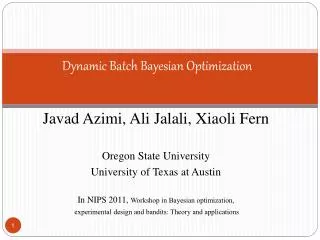
Bayesian Optimization with Experimental Constraints. Javad Azimi Advisor: Dr. Xiaoli Fern PhD Proposal Exam April 2012. Outline. Introduction to Bayesian Optimization Completed Works Constrained Bayesian Optimization Batch Bayesian Optimization

E N D
Bayesian Optimization withExperimental Constraints JavadAzimi Advisor: Dr. Xiaoli Fern PhD Proposal Exam April 2012
Outline • Introduction to Bayesian Optimization • Completed Works • Constrained Bayesian Optimization • Batch Bayesian Optimization • Scheduling Methods for Bayesian Optimization • Future Works • Hybrid Bayesian optimization • Timeline
Bayesian Optimization • We have a black box function and we don’t know anything about its distribution • We are able to sample the function but it is very expensive • We are interested to find the maximizer (minimizer) of the function • Assumption: • lipschitz continuity Introduction to BO Constrained BO Batch BO Scheduling Future Work
Big Picture Select Experiment(s) Posterior Model Current Experiments Run Experiment(s) Introduction to BO Constrained BO Batch BO Scheduling Future Work
Posterior Model (1): Regression approaches • Simulates the unknown function distribution based on the prior • Deterministic (Classical Linear Regression,…) • There is a deterministic prediction for each point x in the input space • Stochastic (Bayesian regression, Gaussian Process,…) • There is a distribution over the prediction for each point x in the input space. (i.e. Normal distribution) • Example • Deterministic: f(x1)=y1, f(x2)=y2 • Stochastic: f(x1)=N(y1,0.2) f(x2)=N(y2,5) Introduction to BO Constrained BO Batch BO Scheduling Future Work
Posterior Model (2):Gaussian Process • Gaussian Process is used to build the posterior model • The prediction output at any point is a normal random variable • Variance is independent from observation y • The mean is a linear combination of observation y Points with high output expectation Points with high output variance
Selection Criterion • Goal: Which point should be selected next to get to the maximizer of the function faster. • Maximum Mean (MM) • Selects the points which has the highest output mean • Purely exploitative • Maximum Upper bound Interval (MUI) • Select point with highest 95% upper confidence bound • Purely explorative approach • Maximum Probability of Improvement (MPI) • It computes the probability that the output is more than (1+m) times of the best current observation , m>0. • Explorative and Exploitative • Maximum Expected of Improvement (MEI) • Similar to MPI but parameter free • It simply computes the expected amount of improvement after sampling at any point MM MUI MPI MEI Introduction to BO Constrained BO Batch BO Scheduling Future Work
Motivating Application:Fuel Cell This is how an MFC works Nano-structure of anode significantly impact the electricity production. e- e- SEM image of bacteria sp. on Ni nanoparticle enhanced carbon fibers. Fuel (organic matter) O2 bacteria H+ H2O Oxidation products (CO2) Cathode Anode • We should optimize anode nano-structure to maximize power by selecting a set of experiment. Introduction to BO Constrained BO Batch BO Scheduling Future Work
Other Applications • Financial Investment • Reinforcement Learning • Drug test • Destructive tests • And … Introduction to BO Constrained BO Batch BO Scheduling Future Work
Constrained Bayesian optimization(AAAI 2010, to be submitted Journal) Introduction to BO Constrained BO Batch BO Scheduling Future Work
Problem Definition(1) • BO assumes that we can ask for specific experiment • This is unreasonable assumption in many applications • In Fuel Cell it takes many trials to create a nano-structure with specific requested properties. • Costly to fulfill Introduction to BO Constrained BO Batch BO Scheduling Future Work
Space of Experiments Averaged Area Average Circularity Problem Definition(2) • It is less costly to fulfill a request that specifies ranges for the nanostructure properties • E.g. run an experiment with Averaged Area in range r1 and Average Circularity in range r2 • We will call such requests “constrained experiments” • Constrained Experiment 1 • large ranges • low cost • high uncertainty about which experiment will be run • Constrained Experiment 2 • small ranges • high cost • low uncertainty about which experiment will be run Introduction to BO Constrained BO Batch BO Scheduling Future Work
Proposed Approach • We introduced two different formulation • Non Sequential • Select all experiments at the same time • Sequential • Only one constraint experiment is selected at each iteration • Two challenges: • How to compute heuristics for constrained experiment? • How to take experimental cost into account?(which has been ignored by most of the approaches in BO) Introduction to BO Constrained BO Batch BO Scheduling Future Work
Non-Sequential • All experiments must be chosen at the same time • Objective function: • A sub set of experiments (with cost B) which jointly have the highest expected maximum is selected, i.e. E[Max(.)] Introduction to BO Constrained BO Batch BO Scheduling Future Work
Submodularity • It simply means adding an element to the smaller set provides us with more improvement than adding an element to the larger set • Example: We show that max (.) is submodular • S1={1, 2, 4}, S2={1, 2, 4, 8}, (S1 is a subset of S2), g=max(.) and x=6 • g(S1, x) - g(S1)=2, g(S2,x)-g(S2)=0 • E[max(.)] over a set of jointly normal random variable is a submodular function • Greedy algorithm provides us with a “constant” approximation bound Introduction to BO Constrained BO Batch BO Scheduling Future Work
Greedy Algorithm Introduction to BO Constrained BO Batch BO Scheduling Future Work
Sequential Policies • Having the posterior distribution of p(y|x,D) and px(.|D) we can calculate the posterior of the output of each constrained experiment which has a closed form solution • Therefore we can compute standard BO heuristics for constrained experiments • There are closed form solution for these heuristics Input space Discretization Level Introduction to BO Constrained BO Batch BO Scheduling Future Work
Budgeted Constrained • We are limited with Budget B. • Unfortunately heuristics will typically select the smallest and most costly constrained experiments which is not a good use of budget • How can we consider the cost of each constrained experiment in making the decision? • Cost Normalized Policy (CN) • Constraint Minimum Cost Policy(CMC) -Low uncertainty -High uncertainty -Better heuristic value -Lower heuristic value -Expensive -Cheap Introduction to BO Constrained BO Batch BO Scheduling Future Work
Cost Normalized Policy • It selects the constrained experiment achieving the highest expected improvement per unit cost • We report this approach for MEI policy only Introduction to BO Constrained BO Batch BO Scheduling Future Work
Constraint Minimum Cost Policy (CMC) • Motivation: • Approximately maximizes the heuristic value • Has expected improvement at least as great as spending the same amount of budget on random experiments • Example: Cost=10 random Cost=5 random Cost=4 random Very expensive: 10 random experiments likely to be better Selected Constrained experiment Poor heuristic value: not select due to 1st condition Introduction to BO Constrained BO Batch BO Scheduling Future Work
Results (1) Real Fuel Cell Cosines Rosenbrock CMC-MEI Introduction to BO Constrained BO Batch BO Scheduling Future Work
Results (2) Real Fuel Cell Rosenbrock Cosines NS Introduction to BO Constrained BO Batch BO Scheduling Future Work
Batch Bayesian Optimization(NIPS 2010) Sometimes it is better to select batch. (JavadAzimi)
Motivation • Traditional BO approach request a single experiment at each iteration • This is not time efficient when running an experiment is very time consuming and there is enough facilities to run up to k experiments concurrently • We would like to improve performance per unit time by selecting/running k experiments in parallel • A good batch approach can speedup the experimental procedure without degrading the performance Introduction to BO Constrained BO Batch BO Scheduling Future Work
Main Idea • We Use Monte Carlo simulation to select a batch of k experiments that closely match what a good sequential policy selection in k steps Given a sequential Policy and batch size k xn1 x31 x21 x11 xn2 x32 x22 x12 x33 xn3 x13 x23 . . . . . . . . . . . . . . . . . . . . . . . . . . . . x3k xnk x2k x1k Return B*={x1,x2,…,xk} Introduction to BO Constrained BO Batch BO Scheduling Future Work
Objective Function(1) • Simulated Matching: • Having n different trajectories with length k from a given sequential policy • We want to select a batch of k experiments that best matches the behavior of the sequential policy • This objective can be viewed as minimizing an upper bound on the expected performance difference between the sequential policy and the selected batch. • This objective is similar to weighted k-medoid Introduction to BO Constrained BO Batch BO Scheduling Future Work
Supermodularity • Example: Min(.) is a supermodual function • B1={1, 2, 4}, B2={1, 2, 4, -2}, f=min(.) and x = 0 • f(B1) -f(B1, x)=1, f(B2)-f(B2, x)=0 • Quiz: What is the difference between submodular and supermodular function? • If the inequality is changed then we have submodular function • The proposed objective function is a supermodular function • The greedy algorithm provides us with an approximation bound Introduction to BO Constrained BO Batch BO Scheduling Future Work
Algorithm Introduction to BO Constrained BO Batch BO Scheduling Future Work
Results (5) Greedy Introduction to BO Constrained BO Batch BO Scheduling Future Work
Scheduling Methods for Bayesian Optimization (NIPS 2011(spotlight))
Extended BO Model Time Horizon h We consider the following: • Concurrent experiments(up to l exp. at any time) • Stochastic exp. durations(known distribution p) • Experiment budget(total of n experiments) • Experimental time horizon h Lab 1 x1 x4 xn-1 Lab 2 x2 x5 x8 x3 x7 xn Lab 3 x6 Lab l Stochastic Experiment Durations • Problem: • Schedule when to start new experiments and which ones to start Introduction to BO Constrained BO Batch BO Scheduling Future Work
Challenges Objective 2: maximize info. used in selecting each experiments (favors minimizing concurrency) Lab 1 x1 x4 x1 x2 xn Lab 2 x2 x5 Lab 3 x3 x6 Lab 4 x7 x4 We present online and offline approaches that effectively trade off these two conflicting objectives Introduction to BO Constrained BO Batch BO Scheduling Future Work
Objective Function • Cumulative prior experiments (CPE) of E is measured as follows: • Example: Suppose n1=1, n2=5, n3=5, n4=2, Then CPE=(1*0)+(5*1)+(5*6)+(2*11)=57 • We found a non trivial correlation between CPE and regret Introduction to BO Constrained BO Batch BO Scheduling Future Work
Offline Scheduling • Assign start times to all n experiments before the experimental process begins • The experiment selection is done online • Two class of schedules are presented • Staged Schedules • Independent Labs Introduction to BO Constrained BO Batch BO Scheduling Future Work
Staged Schedules • There are N stage and each stage is represent as <ni,di> such that • CPE is calculated as: • We call an schedule uniform if |ni-nj|<2 n1=4 n2=3 n3=4 n4=3 x1 x5 x8 x12 x2 x6 x9 d3 x13 d1 d2 d4 x3 x7 x10 x14 x4 x11 h • Goal: finding a p-safe uniform schedule with maximum number of stages. Introduction to BO Constrained BO Batch BO Scheduling Future Work
Staged Schedules: Schedule Introduction to BO Constrained BO Batch BO Scheduling Future Work
Independent Lab (IL) • Assigns miexperiment to each lab isuch that • Experiments are distributed uniformly within the labs • Start times of different labs are decoupled • The experiments in each lab have equal duration to maximize the finishing probability within horizon h • Mainly designed for policy switching schedule x11 x12 x13 x14 Lab1 x21 x22 x23 x24 Lab2 Lab3 x31 x32 x33 Lab4 x41 x42 x43 h Introduction to BO Constrained BO Batch BO Scheduling Future Work
Online Schedules • p-safe guarantee is fairly pessimistic and we can decrease the parallelization degree in practice • Selects the start time of experiments online rather than offline • More flexible than offline schedule Introduction to BO Constrained BO Batch BO Scheduling Future Work
Baseline online Algorithms • Online Fastest Completion policy (OnFCP) • Finish all of the n experiments as quickly as possible • Keeps all l labs busy as long as there are experiments left to run • Achieves the lowest possible CPE • Online Minimum Eager Lab Policy (OnMEL) • OnFCP does not attempt to use the full time horizon • use only klabs, where k is the minimum number of labs required to finish n experiments with probability p Introduction to BO Constrained BO Batch BO Scheduling Future Work
Policy Switching (PS) • PS decides about the number of new experiments at each decision step • Assume a set of policies or a policy generator is given • The goal is defining a new policy which performs as well as or better than the best given policy at any state s • The i-th policy waits to finish iexperiments and then call offIL algorithm to reschedule • The policy which achieves the maximum CPE is returned • The CPE of the switching policy will not be much worse than the best of the policies produced by our generator Introduction to BO Constrained BO Batch BO Scheduling Future Work
Experimental Results Setting: h=4,5,6; pd=Truncated normal distribution, n=20 and L=10 Best Performance Best CPE in each setting Introduction to BO Constrained BO Batch BO Scheduling Future Work
Future Work Introduction to BO Constrained BO Batch BO Scheduling Future Work
Traditional Approaches • Sequential: • Only one experiment is selected at each iteration • Pros: Performance is optimized • Cons: Can be very costly when running one experiment takes long time • Batch: • k>1 experiments are selected at each iteration • Pros: k times speed-up comparing to sequential approaches • Cons: Can not performs as well as sequential algorithms Introduction to BO Constrained BO Batch BO Scheduling Future Work
Batch Performance (Azimi et.al NIPS 2010) k=5 k=10 Introduction to BO Constrained BO Batch BO Scheduling Future Work
Hybrid Batch • Sometimes, the selected points by a given sequential policy at a few consequent steps are independent from each other • Size of the batch can change at each time step (Hybrid batch size) Introduction to BO Constrained BO Batch BO Scheduling Future Work
First Idea(NIPS Workshop 2011) x2 x3 x1 Based on a given prior (blue circles) and an objective function (MEI), x1 is selected To select the next experiment, x2, we need, y1=f(x1) which is not available The statistics of the samples inside the red circle are expected to change after observing at actual y1 We set y1 =M and then EI of the next step is upper bounded If the next selected experiment is outside of the red circle, we claim it is independent fromx1 Introduction to BO Constrained BO Batch BO Scheduling Future Work
Next • Very pessimistic to set Y=M and then the speedup is small • Can we select the next point based on any estimation without degrading the performance? • What is the distance of selected experiments in batch and the actual selected experiments by sequential policy? Introduction to BO Constrained BO Batch BO Scheduling Future Work
TimeLine • Spring 2012: Finishing the Hybrid batch approach • Summer 2012: Finding a job and final defend (hopefully ) Introduction to BO Constrained BO Batch BO Scheduling Future Work
And • I would like to thank Dr. Xaioli Fern and Dr. Alan Fern Introduction to BO Constrained BO Batch BO Scheduling Future Work