Download
1 / 16
170 likes | 186 Views
PIXEL SCANS. Measuring Data. Measure last point before graphs cuts off at 1/10 ³. For spread of data, imagine fitting curve and take point where it would cross X axis. For larger spreads of data (see opposite), fit cubic polynomial. Mask Scanning. 9 x 9 Mask Scanned 3 x 3 Aperture

E N D
Measuring Data • Measure last point before graphs cuts off at 1/10³. • For spread of data, imagine fitting curve and take point where it would cross X axis. • For larger spreads of data (see opposite), fit cubic polynomial.
Mask Scanning • 9 x 9 Mask Scanned • 3 x 3 Aperture • 60% Intensity • 50μm step size • 1064nm Wavelength • 25Hz Firing Frequency • Continuous Firing • Scan Type: mpsAnalysis Threshold 149 • Scanned Between 50 and 350 units.
Mask Scanning – 3D • Data Plotted In 3D for aesthetics. • Cut Off Point Measured By Eye, defined as when no hits are recorded with more than 1/10³ frequency.
Mask Scanning: Histogram • Gaussian Fitted Ignoring Saturated Data Points. • Fitted by eye so may not be optimum
Mask Scans Other Region • Another region was also scanned, 6mm down on sensor. • Prob statistic for green histogram is 0.1688. Mean = 186.7 ± 4.3. Sigma = 32.21 ± 4.11
Pedestal Adjustment • Pedestals For each Pixel Subtracted And Data Replotted
Pedestal Adjusted Histogram • Gaussian Again Fitted By Eye. • Histogram Does Not Include Saturated Pixels - 72 points.
Intensity • Automated Scans of Intensity For Several Pixels • 30-100% Alternating Steps of 2% and 3%. • Scanned between 0 and 500 units.
Does Turning Laser Off and On Make A Difference? NO SIGNIFICANT DIFFERENCE
Alignment Data • Scanned In Alternating 5 and 6 micron steps, over whole of Pixel (28,143). • 2 x 2 Aperture • 1 x 1 Mask over chosen pixel • 60% Intensity • (All other settings same as for Mask Scanning) • Coordinates arbitrary to allow ROOT plots.
Alignment Plots Looks As Though Laser Is Out of Focus!!!
Focused Alignment Scans • Scanned Along X Axis Through Centre of Four Pixels (Separate 1 x 1 Mask for each) • 2μm steps. • Pixel (29,143) best displayed twin peaks.
Pixel (29,143) Alignment • Scanned along Y axis (through maximum point from earlier scan) to find Diode. • Then along X axis, through maximum Point from Y Axis Scan.
END More data is at SpiderWiki http://hepilc01.pp.rl.ac.uk/spiderwiki