Download
1 / 25
310 likes | 1.31k Views
Spike sorting Tutorial. Rodrigo Quian Quiroga. Problem: detect and separate spikes corresponding to different neurons. Outline of the method:. I - Spike detection: amplitude threshold. II - Feature extraction: wavelets. III - Sorting: Superparamagnetic clustering. Goals:.

E N D
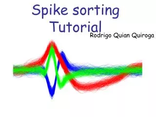
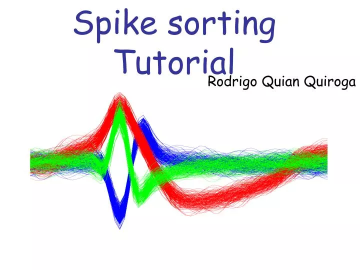
Spike sorting Tutorial Rodrigo Quian Quiroga
Problem:detect and separate spikes corresponding to different neurons
Outline of the method: I - Spike detection: amplitude threshold. II - Feature extraction: wavelets. III - Sorting: Superparamagnetic clustering. Goals: • Algorithm for automatic detection and sorting of spikes. • Suitable for on-line analysis. • Improve both detection and sorting in comparison with previous approaches.
This tutorial will show you how to do spike sorting using: • Thewave_clusgraphic user interface. • The batch files Get_spikes and Do_clustering.
Getting started… • Add the directory wave_clus with subfolders in your matlab path (using the matlab File/Set Path menu) • Type wave_clus in matlab to call the GUI. • Choose DataType simulator and load the file C_Easy1_noise01_short (in the subdir wave_clus/Sample_data/Simulator) using the Load button.
Now you are ready to start playing withwave_clus … • This is a 10 sec. segment of simulated data. • First, choose the option plot_average to plot the average spike shapes (+/- 1 std). Then choose to plot the spike features. • There may be some spikes unassigned in cluster 0. Go back to plot_all and use the Force button to assign them to any of the clusters. Better? • Now change the temperature. At t=0 you will get a single cluster, for large t’s you may get many clusters (if the parameter min_clus allows it). • Save the results using the Save clusters button. Load the output file times_C_Easy1_noise01.mat. Cluster membership is saved in the first column of the variable cluster_class. The second column gives the spike times. • You can also change the isi histogram plots using the max and step options. • Finally check the parameters used in the Set_parameters_simulation file in the wave_clus/Parametes_files (just type ‘open set_parameters_simulation’ in matlab).
Playing with the spike features… • Load the file C_Difficult1_noise015 using again the DataType: Simulator. • Use the Spike features option
Seeing the clusters… • You may, however, get something different cause SPC is a stochastic clustering method. If you don’t get the 3 clusters, you may have to change the temperature. • The are 3 different spike shapes, but you don’t see three clear clusters. That’s because wave_clus plots in the main window the first 2 wavelet coefficients. • You can see the rest of the projections by clicking the Plot all projections button
It would look like this… Clusters separate clearly in some projections
Using Principal ComponentAnalysis • Now do the same using PCA. Open set_parameters_simulation and select features = ‘pca’ instead of features = ‘wav’ (don’t forget to set it back to ‘wav’ when you are done!). • Load again the data C_Difficult1_noise015.
Why PCA does so bad here? • As you see, there’s now only one single cluster (and for no temperature you can split it into 3!). You have just replicated the results of Fig. 8 of the Neural Computation paper (see reference at the end). • In this dataset the spike shapes are very similar, and their differences are localized in time. Do to its excellent time-frequency resolution, wavelets does much better. • Also, don’t forget that PCA looks for directions of maximum variance, which are not necessarily the ones offering the best separation between the clusters. Wavelets combined with the KS test (see paper) looks for the coefficients with multimodal distribution, which are very likely the ones offering the best separation between the clusters. • As a summary, in the Neural Computation paper it is shown for several different examples of simulated data a better performance of wavelets in comparison to PCA.
You are now ready for real data! • You will now load a ~30’ multiunit recording from a human epilepsy patient. The data was collected at Itzhak Fried’s lab at UCLA. • Intracranial recordings in these patients (refractory to medication) are done for clinical reasons in order to evaluate the feasibility of epilepsy surgery. • Load the file CSC4 using the DataType: CSC (pre-clustered). Using the (pre-clustered) option you will load data that has already been clustered using the batch file Do_clustering_CSC. If you want to start from scratch use the CSC option. • Check the settings in the Set_parameters_CSC file. If you have a Neuralynx system you can already use the CSC and Sc options for your own data. • BTW, there should be a few cool publications coming up using these human data. If you’re interested check www.vis.caltech.edu/~rodri/publications in the near future or email me.
Playing with it… • Again, you can change the temperature, force the clustering, see the spike features, etc. Remember that everything is much faster is you use Plot_average instead of Plot_all. • You can also zoom into the data using the Tools menu. • You may also want to fix a given cluster by using the fix button. This option is useful for choosing clusters at different temperatures or for not forcing all the clusters together.
One further example: • Sometimes clusters appear at different temperatures • In the following example we give a step-by-step example of a clustering procedure using the fix button
Step 1: Fix cluster 2 at low T Step 3: Check features Step 2: Change to T2 Step 4: Fix clusters 2 and 3
Step 5: Change to T3 Step 6: Re-check features Step 7: Push the Force button This is how the final clustering looks like! Note that after forcing the green cluster is not as clean as before.
Clustering your own data… • Most likely you’ll end up using the ASCII DataType option for your data. • If you have continuous data, it should be stored as a single vector in a variable data, which is saved in a .mat file. Look for the file test.mat for an example. This data should be loaded using the ASCII option or the ASCII (pre-clustered) if you have already clustered it with the Do_clustering batch file. • If you have spikes that have already been detected, you should use the ASCII spikes option. The spikes should be stored in a matrix named spikes in a .mat file. The file test1_spikes.mat gives an example of the format. • You can set the optimal parameters for you data in the corresponding Set_parameters_ascii (or ascii_spikes) file. Most important, don’t forget to set the sampling rate sr! • Important note: To save computational time, if you have more than 30000 spikes in your dataset, by default these will be assigned by template matching with the batch clustering code (this can be changed in the set_parameters file). With the GUI, they will stay in cluster 0 and they should be assigned to the other clusters using the Force button. Note that if you don’t do this you will be just processing the first 30000 spikes.
Using the batch files… • There are two main batch files: Get_spikes (for spike detection) and Do_clustering (for spike sorting). Parameters are set in the first lines.They both go through all the files set in Files.txt. • Unsupervised results will be saved and printed (either in the printer or in a file), but can be later changed with the GUI. For changing results, you have to load the file with the (pre-clustered) option. The nice thing is that results for all temperatures are stored, so changing things with the GUI mainly implies storing a different set of results rather than doing the clustering again. Note that using the GUI for clustering (e.g. with the ASCII option) does not store the clustering results for future uses.
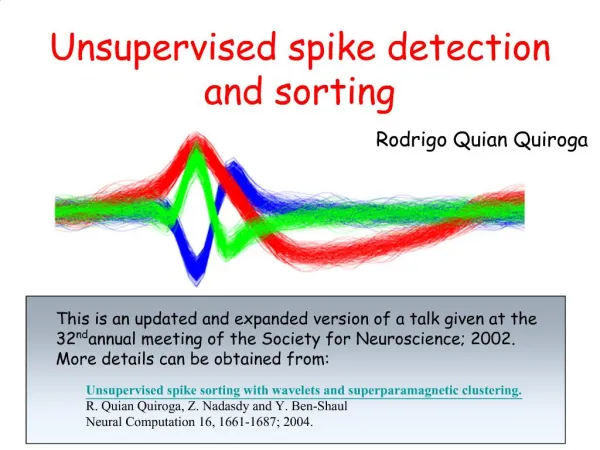
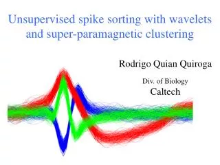
You are now a clustering expert! • If you want further details on the method, check: Unsupervised spike sorting with wavelets and superparamagnetic clustering R. Quian Quiroga, Z. Nadasdy and Y. Ben-Shaul. Neural Computation 16, 1661-1687; 2004. • If you want to keep updated on new versions, give me some comments or feedback on how wave_clus works with your data (I would love to hear about it), etc. please email me at: rodri@vis.caltech.edu • Good luck and hope it’s useful!