Download
1 / 38
380 likes | 538 Views
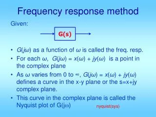
Frequency Resp. method. Given: G ( j ω ) as a function of ω is called the freq. resp. For each ω , G ( jω ) = x ( ω ) + jy ( ω ) is a point in the complex plane As ω varies from 0 to ∞, the plot of G ( jω ) is called the Nyquist plot. Can rewrite in Polar Form:

E N D
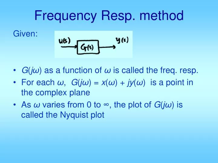
Frequency Resp. method Given: • G(jω) as a function of ω is called the freq. resp. • For each ω, G(jω) = x(ω) + jy(ω) is a point in the complex plane • As ω varies from 0 to ∞, the plot of G(jω) is called the Nyquist plot
Can rewrite in Polar Form: • |G(jω)| as a function of ω is called the amplitude resp. • as a function of ω is called the phase resp. • The two plots: With log scale-ω, are Bode plot
To obtain freq. Resp from G(s): • Select • Evaluate G(jω) at those to get • Plot Imag(G) vs Real(G): Nyquist • or plot With log scale ω • Matlab command to explore: nyquist, bode
To obtain freq. resp. experimentally: • Select • Given input to system as: • Adjust A1 so that the output is not saturated or distorted. • Measure amp B1 and phase φ1 ofoutput:
Then is the freq. resp. of the system at freq ω • Repeat for all ωK • Either plot or plot
System type, steady state tracking, & Bode plot C(s) Gp(s) R(s) Y(s)
As ω → 0 Therefore: gain plot slope = –20N dB/dec. phase plot value = –90N deg
If Bode gain plot is flat at low freq, system is “type zero” Confirmed by phase plot flat and 0° at low freq Then: Kv = 0, Ka = 0 Kp = Bode gain as ω→0 = DC gain (convert dB to values)
Steady state tracking error Suppose the closed-loop system is stable: If the input signal is a step, ess would be = If the input signal is a ramp, ess would be = If the input signal is a unit acceleration, ess would be =
N = 1, type = 1 Bode mag. plot has –20 dB/dec slope at low freq. (ω→0) (straight line with slope = –20 as ω→0) Bode phase plot becomes flat at –90° when ω→0 Kp= DC gain → ∞ Kv = K = value of asymptotic straight line at ω = 1 =ws0dB =asymptotic straight line’s 0 dB crossing frequency Ka = 0
Example Asymptotic straight line ws0dB ~14
The matching phase plot at lowfreq. must be → –90° type = 1 Kp= ∞ ← position error const. Kv = value of low freq. straight line at ω = 1 = 23 dB ≈ 14 ← velocity error const. Ka = 0 ← acc. error const.
Steady state tracking error Suppose the closed-loop system is stable: If the input signal is a step, ess would be = If the input signal is a ramp, ess would be = If the input signal is a unit acceleration, ess would be =
N = 2, type = 2 Bode gain plot has –40 dB/dec slope at low freq. Bode phase plot becomes flat at –180° at low freq. Kp= DC gain → ∞ Kv = ∞ also Ka = value of straight line at ω = 1 = ws0dB^2
Example Ka ws0dB=Sqrt(Ka) How should the phase plot look like?
Steady state tracking error Suppose the closed-loop system is stable: If the input signal is a step, ess would be = If the input signal is a ramp, ess would be = If the input signal is a unit acceleration, ess would be =
System type, steady state tracking, & Nyquist plot C(s) Gp(s) As ω → 0
Type 0 system, N=0 Kp=lims0 G(s) =G(0)=K Kp w0+ G(jw)
Type 1 system, N=1 Kv=lims0sG(s) cannot be determined easily from Nyquist plot winfinity w0+ G(jw) -j∞
Type 2 system, N=2 Ka=lims0 s2G(s) cannot be determined easily from Nyquist plot winfinity w0+ G(jw) -∞
Margins on Bode plots In most cases, stability of this closed-loop can be determined from the Bode plot of G: • Phase margin > 0 • Gain margin > 0 G(s)
If never cross 0 dB line (always below 0 dB line), then PM = ∞. If never cross –180° line (always above –180°), then GM = ∞. If cross –180° several times, then there are several GM’s. If cross 0 dB several times, then there are several PM’s.
Example: Bode plot on next page.
Example: Bode plot on next page.
Where does cross the –180° lineAnswer: __________at ωpc, how much is • Closed-loop stability: __________
crosses 0 dB at __________at this freq, • Does cross –180° line? ________ • Closed-loop stability: __________
Margins on Nyquist plot Suppose: • Draw Nyquist plot G(jω) & unit circle • They intersect at point A • Nyquist plot cross neg. real axis at –k