Download
1 / 57
610 likes | 1.02k Views
Modeling and Simulation - 1. Instructor: Giampiero Pecelli e-mail: Giampiero.Pecelli@mikkeliamk.fi e-mail: giam@cs.uml.edu Office Phone: Office: Office Hours:1:00PM-4:00PM Course Materials : www.cs.uml.edu/~giam/mikkeli

E N D
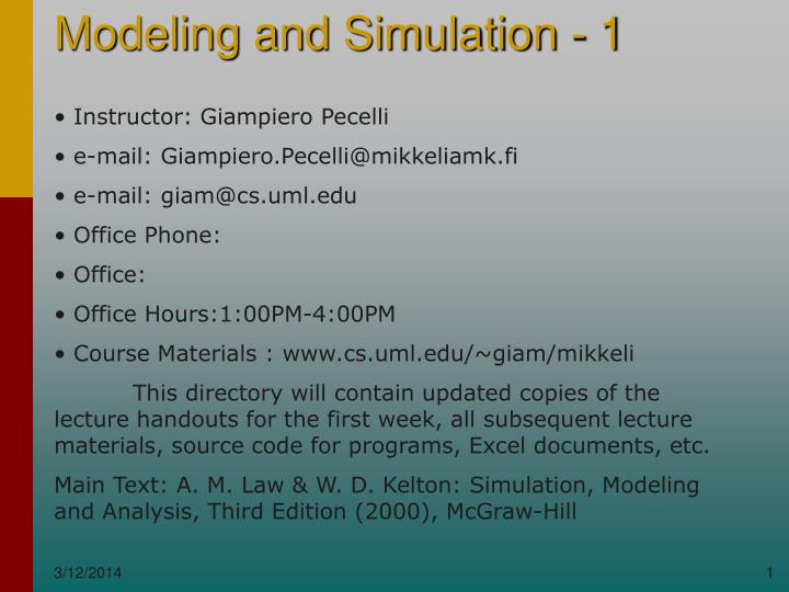
Modeling and Simulation - 1 • Instructor: Giampiero Pecelli • e-mail: Giampiero.Pecelli@mikkeliamk.fi • e-mail: giam@cs.uml.edu • Office Phone: • Office: • Office Hours:1:00PM-4:00PM • Course Materials : www.cs.uml.edu/~giam/mikkeli This directory will contain updated copies of the lecture handouts for the first week, all subsequent lecture materials, source code for programs, Excel documents, etc. Main Text: A. M. Law & W. D. Kelton: Simulation, Modeling and Analysis, Third Edition (2000), McGraw-Hill
Modeling and Simulation - 1 Why Modeling & Simulation? How Modeling & Simulation? What Modeling & Simulation?
Modeling and Simulation - 1 • WHY? We need to conduct experiments "on some reality" and the reality - although pre-existing - is not available for our experiments. Examples: a) a busy network of computers that cannot be taken over just for the experiment; b) a busy superhighway system on which we want to "change the rules of traffic"; c) a chemical plant whose production cannot be stopped so that "we can tinker with it"; etc..
Modeling and Simulation - 1 • What characteristic do these example share? They simply have to do with our lack of access to an existing artifact: the simulation allows us to construct a useful model of the artifact, that we can then use as though it were the inaccessible artifact. The goal is to determine whether a planned change to the USE of the artifact can be implemented while producing the desired results and no undesired ones. A more specific example would be the introduction of the use of a "group productivity package", like Lotus Notes or a Configuration and Version Manager for a software producing organization. In both cases the traffic patterns - and bottlenecks - in a LAN might not be predictable without extensive testing, and any meaningful REAL testing will result in many lost productivity hours for the whole group or organization that is adopting the package.
Modeling and Simulation - 1 • A second set of examples. These have to do with the absence of an appropriate artifact. Here are some examples: a) An automobile frame that must meet certain stiffness and crushability criteria, while also meeting geometry, materials, production method and weight constraints; b) An algorithm to manage certain types of (not yet available?) traffic in networks with as yet non-existent (but likely, or already possible) properties (e.g., 20 TH bandwidth); c) The design of drugs with special properties;
Modeling and Simulation - 1 • What characteristic do these example share? There is NO artifact on which to perform experiments, and the construction of any such artifact is not feasible (too expensive - current technology is too immature - too dangerous) without knowledge that the finished artifact will behave (with sufficiently high probability) as desired. There MAY exist earlier versions of similar artifacts, with different characteristics, that MIGHT be used as guides for the design of a simulation, but with no guarantee that the results of the simulation can be compared to "real" data in the regions of interest.
Modeling and Simulation - 1 • Simulation (Shannon): The process of designing a computerized model of a system (or process) and conducting experiments with this model for the purpose either of understanding the behavior of the system or of evaluating various strategies for the operation of the system. System: an orderly collection of logically related principles, facts or objects that act and interact together toward the accomplishment of some logical end. Process: a method of doing something involving multiple steps and operations.
Modeling and Simulation - 1 Ways to study a system. System Experiment with the actual system Experiment with a model of the system Physical model Mathematical model Analytical solution Simulation
Modeling and Simulation - 1 • Some terminology. A) System Environment: the collection of external factors capable of causing a change in the system. B) State of a System: the minimal collection of information with which the future behavior of a system can be reliably (uniquely?) predicted. C) Activity: any event that causes a State Change. D) Endogenous Activity: one occurring inside the system. E) Exogenous Activity: one occurring outside the system.
Modeling and Simulation - 1 F) Continuous System (Model): one in which the quantities of interest are represented by continuous variables (e.g., distances between cars on a highway). Sometimes a discrete system (packets in a network) can be treated as a continuous model. G) Discrete System (Model): one in which the quantities of interest are represented by discrete-valued variables (e.g., number of cars on a highway, number of cars queued up at the toll-booth), sometimes integers, but not always so. The change in values is instantaneous (discontinuity…) F) Hybrid System (Model): one in which both discrete and continuos variables appear (e. g., number of and distances between cars) and are of interest. These are probably the most common.
Modeling and Simulation - 1 G) Deterministic System (Model): one in which the next state is uniquely determined by the current state. Examples: Classical Mechanics; anything that can be adequately modeled via Newtonian Mechanics: hit the brakes of your car under exactly controlled conditions and the distance it takes for you to come to a stop can be exactly predicted. Deterministic Automata. H) Stochastic System (Model): one in which the next state is only probabilistically determined by the current state - there are multiple possible next states that can occur subsequent to the same activity, each with a given probability. Examples: Quantum Mechanical phenomena. Markov Chains. Non-deterministic automata.
Modeling and Simulation - 1 I) Dynamic Model. Represents a system as it evolves in time. Most of the models we will study and program are of this type. J) Static Model. Represents a system at one particular time - or represents a system for which time is not a parameter. We will see a Monte Carlo simulation that computes the area of a circle.
Modeling and Simulation - 1 The Stages of a Simulation Project. • Planning a) Problem Formulation: what is it and what do I want to do with it? b) Resource Estimation: time, people and money. c) System and Data Analysis • Modeling a) Model Building: find relationships. b) Data Acquisition: find and collect appropriate data. c) Model Translation: program and debug.
Modeling and Simulation - 1 • Verification/Validation a) Verification: does the PROGRAM execute as intended? b) Validation: does the PROGRAM represent reality as intended? • Application a) Experimentation: run it! b) Analysis: how do I analyze and interpret the results? c) Implementation/Documentation: how do I implement the decisions resulting from the simulation, and how do I document the model and its use?
Modeling and Simulation - 1 • Performance Measures. What is it that we are measuring? What (statistical) properties of the "measured" are we interested in? For example: maximum, minimum, totals, mean, variance, higher moments, specific frequency distribution, interarrival times, service times, lengths of queues, loss rates, error rates, etc.
Modeling and Simulation - 1 Advantages of Simulation. a) it permits controlled experimentation. you KNOW what parameters are being changed. b) it permits time compression. e.g., weather forecasting... c) it permits sensitivity analysis (change input vars) d) it does not disturb the real system. which may not even exist, anyway. e) it is an effective training tool. you are not likely to crash a flight simulator, or a big chunk of the Internet.
Modeling and Simulation - 1 Steps in a Simulation Study - a Flowchart from the text. 1. Formulate problem and plan the study 7. Design Experiments 2. Collect data and define the model 8. Make Production runs 3. Conceptual model valid? 9. Analyze output data No 10. Document, present and use results Yes 4. Construct a computer program and verify 5. Make Pilot Runs 6. Programmed model valid? Yes No
Modeling and Simulation - 1 Through all the stages make sure that: a) you are in contact will all the appropriate people, both technical and managerial; keep the contacts active; b) make sure that what you think you understood is what the other side thinks it understands; c) make sure that the people who want the system know what they want and its relationship to what they are getting;
Modeling and Simulation - 1 My own current interest: How do you experiment in a meaningful way with algorithms whose theoretical properties can be predicted? Most of these algorithms attempt to provide management for traffic which is, as yet, not well understood, in networks with characteristics that don't yet exist. Qualitative and quantitative mathematical predictions can be obtained only under considerably simplified assumptions on the system being studied. How well will these predictions compare with reality? Can simulation provide a reasonable answer? Many engineers construct an algorithm that will exhibit SOME desired behaviors, run a few simulations, call it quits and send a paper out - or build a system and graft it onto an existing larger system. Is this a prescription for nonsense? Or worse?
Modeling and Simulation - 1 Some Examples of Simulations and Simulation Systems. Before we approach the systematic study of simulation environments and a simulation methodology, we will look at a number of relatively simple examples. Some of these examples will be "classical", in the sense that they make use of completely deterministic models (and yet can show quite chaotic behavior) with fixed time steps, some will be a little more "modern" - in the sense that they rely on computer methods to introduce event-driven system updates. There are two primary time advance mechanisms: one is the fixed-increment time advance, often used for physical or biological modeling; the second is the next-event time advance, which is commonly used for discrete event simulation, where the times at which events occur are not "naturally" uniformly spaced. Since two of the three examples in this section are of the first type, we will present a description of the general method before we go on.
Modeling and Simulation - 1 An Aside on Fixed-Increment Time Advance. With this approach, the simulation clock is advanced in fixed increments, say Dt. After the clock update, the system checks if any events should have occurred during the previous Dt interval. Any such are considered to have occurred at the end of the interval, are processed as such, and the system state and counters are updated accordingly. 0 e1 Dt 2Dt e2 e3 3Dt e4 4Dt e1 occurs at time Dt, e2 and e3 occur at time 3Dt, etc… This works well for those simulations where the events really are synchronized with the clock pulses, less well otherwise.
Modeling and Simulation - 1 A simple example: the logistic equation (variant). In the study of biological populations, a certain simple equation has seen much use over the decades. It seems to model a number of populations with reasonable accuracy, it is easily modified to include various "tweaks", and it shows all kinds of interesting behavior. The best kind of population to be modeled is one of "insects with non-overlapping generations" - one generation is dead before the next one is hatched. It may or may not model the Gypsy Moth (a moth that appears in the early Spring, in caterpillar form eats all the new growth from many species of trees, and then becomes a moth and lays eggs that will hatch during the subsequent Spring). If the moth appears in sufficiently large quantities over a period of three or more years, substantial die-offs of trees will occur, since their having to re-grow a full set of leaves twice in a season leaves them weakened, and, eventually, incapable of recovery.
Modeling and Simulation - 1 The Equation. Where: • X(n) is the population at generation n. • r is a "reproduction factor" intrinsic to the species. • K is the "environmental carrying capacity" - the maximum number of individuals the environment can support. In terms of our Gypsy Moth example, r is related to the number of descendant of each individual that are likely to reach the stage when they eat foliage; K is the amount of biomass (foliage) available for feeding; X(n) is the number of Gypsy Moths in the local population.
Modeling and Simulation - 1 Notice the product term: reproduction depends on the number of individuals in the current population and on the amount of pressure they put on the environment: a small population will reproduce at maximum rate, a large population (near the maximum supportable by the environment) will reproduce at a low rate. The maximum value for the right hand side - and thus the largest possible next generation will occur for X(n) = K/2. Values of r below 1 will lead to a disappearing population, while values above 4 will lead to a model breakdown. This is a fairly standard model - others take into account various types of efficiency, etc., but the general idea is the same.
Modeling and Simulation - 1 In order for us to be able to use this equation to predict the behavior of the population at generation n, we need to know several things: • the initial population X(0); • the value of K; • the value of r. A quick look allows us to simplify matters a little - in simulation and modeling you are always on the lookout for parameters that can be ignored (or coalesced into a single expression)- if we replace X(n) by Y(n)*K, we end up with an equation without K. Y(n) will take values between 0 and 1, and we can reconstruct X(n) by simply multiplying Y(n)*K. There is something slightly wrong with this, but not impossibly so - what is it?
Modeling and Simulation - 1 The equation becomes: We have a usable relationship, and we need to set up a simulation to try to study the evolution of populations - we would have to check that the predictions of the model agree with experimental results. How do we do that? A common, although quite powerfulenvironment is provided by the spreadsheet Excel. How do we use it? We need two cells for the parameter r and the initial condition Y(0), we need one cell in which we write the formula to move from the first (zeroth?) generation to the next and then use the fact that copying formulae in Excel allows for automatic updating of variable indices.
Modeling and Simulation - 1 The initial population Y(0) is taken to be 1% of the environmental carrying capacity, with a reproductive factor of r = 4. The choices of these values do not appear motivated by much of anything - they give rise to a population whose evolution can be plotted against the number of generations:
Modeling and Simulation - 1 This does not appear very useful - too many of the projected populations are near 0 or 1. This is where the normalization can create problems: populations are made up of discrete individuals - you can't have viable offspring from 1/2 of a Gypsy Moth, but you CAN have a non-zero value for the next generation, as given by the formula, unless you take care… Let's change some of the parameters. If we start with r small (say 1.5), and increase it slowly, we find that the terminal population becomes constant - with values that seem to depend on r, all the way to - approximately - r = 3. For r > 3, the system shows oscillations, of greater and greater period as r increases; for r > 3.6 the system shows what appears to be random or chaotic behavior, becoming more chaotic as r increases. Our first try, at r = 4, was well into the chaotic region...
Modeling and Simulation - 1 The point to be made is that simulation runs cannot give us the parameter values where qualitative changes will occur: they will give us approximations, which may be all we can achieve, but leave us with the problem of determining exactly what kinds of behaviors we can expect. They also do not let us conclude that we have observed all possible types of behaviors. For the next step, an analytical approach is necessary. This isn't to say that it is always done: there may be many reasons why the study will stop at a series of simulation runs. The most serious one is that the model may be so complex that no analytical approach is likely to provide useful information. Fortunately, this is not the case for the logistic equation.
Modeling and Simulation - 1 Step 1. The constant solution. We can obtain the value of the constant solution by first observing that a constant solution must satisfy the condition X(n) = X for all n ≥ 0. This leads to the equation which has the solution X(n)=0 for all n ≥0, which is not very useful, and, for r > 1, the solution We now have formulae for the constant solutions shown in the simulations - the analytic values match the simulation ones. The simulation also showed that, for r > 3, we should expect to see oscillatory behavior. Another way of describing this is that the constant solution has changed from asymptotically stable to unstable.
Modeling and Simulation - 1 Step 2. First Order Effects, or the Linearized Equation. The next step involves changing variables so that the constant solution of interest lies at the origin, and then observing that, near the origin, all terms of degree higher than one will contribute little to the behavior near the origin, when compared to constant or degree one terms. Performing the change of variables gives the equation (after simplification): where Y(n) represents the deviation from the constant solution. Dropping the terms of degree higher than 1, we have the Linearized Equation: which we can solve in closed form.
Modeling and Simulation - 1 It is easy to see that |2 - r| < 1 (i.e.,1 < r < 3) implies that Y(n)-> 0 as n -> ∞, and that the constant solution is asymptotically stable; r = 3 implies that Y(n) oscillates between two values, ±Y(0), while r > 3 implies that Y(n) increases exponentially and thus that the constant solution is not stable. This confirms the tentative conclusion based on the simulation results. One can use the higher order terms to obtain more information - the techniques to do so are beyond the scope of this course.
Modeling and Simulation - 1 At this point we have a model, some prediction from the model, and an analytical study of the model. How do we determine whether this model is modeling the desired system? We have, essentially, three things: 1) The initial population. We might be able to find this value experimentally, over several population cycles. 2) The reproduction rate. This should also be experimentally obtainable. It may take several observations. 3) The environmental carrying capacity. We hid it, but, in order to "normalize" the population, we have to resurrect it as an experimentally determinable quantity. Again several observations might be necessary.
Modeling and Simulation - 1 We will end up with three sets of observations, representing three "statistical populations": the population of possible initial values; the population of reproductive rates; and the population of carrying capacities. These populations will have means, variances, probability distributions, etc. From the measurements we should be able to use statistical techniques to obtain values to use in the simulation engine. For each such triplets of initial values and parameters, the simulation engine outputs a sequence of populations. We can measure the population sequence over "many" generations, and we can use statistical techniques to determine properties of the sequence. We can use statistical techniques to determine whether the sequences produced by the model are sufficiently close to the sequences produced by actual observation to conclude that the model is "good enough" for our purposes.
Modeling and Simulation - 1 A more complex example: competition between two populations. This particular type of model was investigated beginning around 1925 by Lotka, Volterra, and others - in the context of population biology, but with the possibility of applying the results to economic modeling and other areas. The models are instructive and will let us show some of the simpler analytic techniques. The presentation is partially taken from H. T. Davis, Introduction to Nonlinear Differential and Integral Equations, Dover Pub., New York, 1962.
Modeling and Simulation - 1 We assume two interacting populations, A and B, consisting, respectively, of NA and NB individuals. Without any interference, population A (prey) would increase exponentially without bound according to the growth law while population B (predator) would decrease exponentially according to the law In a common, bounded environment, individuals of the two species will encounter one another proportionally to NA * NB . A certain proportion of these encounters will result in the death of a member of species A (the prey), and they will contribute to the growth of species B. We assume the contribution to be immediate (no long gestation period), and also proportional to the number of encounters. We end up with the system of differential equations:
Modeling and Simulation - 1 Question 1. Does this system of Ordinary Differential Equations have a non-trivial constant solution? Non-trivial means that both populations are positive for all time. Since a constant solution has an identically vanishing derivative, we must look for solutions to the (nonlinear) algebraic system: It is easy to see that the system has the pair of solutions: The second pair satisfies our conditions.
Modeling and Simulation - 1 Question 2. What is the nature of this constant solution? More precisely are there any values of the parameters a, b, c, d, for which the constant solution is asymptotically stable? unstable? In the first case, solutions starting near the constant one will evolve becoming nearer and nearer it as time progresses. In the second case we should expect either some kind of "explosive behavior" or oscillations. Explosive behavior is not overly likely in "real populations", since they have multiple checks and balances, so oscillation is the most likely form that instability will take. How can we determine this? Step 1. Change variables in the system of ODEs: nA(t) and nB(t) represent the deviation from the constant solution, and will be treated as "small quantities".
Modeling and Simulation - 1 We have the non-linear system: Step 2. Linearize the system - drop all terms of degree higher than 1. This gives the new system:
Modeling and Simulation - 1 We look for solutions of the form: Substituting into the differential equation, we obtain: Which reduces to:
Modeling and Simulation - 1 This matrix equation can have a nonzero solution - i.e.nonzero nA(0) and nB(0) - only if the determinant of the coefficient matrix vanishes: This has two distinct imaginary solutions : and linearly independent vector solutions of the matrix equation corresponding to the zeros of the determinant: Finally, two linearly independent solutions for the linearized system of differential equations.
Modeling and Simulation - 1 The unfortunate result is that the linearized system possesses only circular motions: no asymptotic stability for the constant solution - the nonlinear terms will really determine the behavior, since no transition from stability to instability can ever occur as the parameters change. As it turns out, there are other methods by which one can carry out an analytic study of the system, and obtain a fairly complete picture of the behavior of the two populations. At this point, we will instead react as though this were "too complex a system to study analytically" and look for some other attack. The simulation attack may be the appropriate one. How do we do this?
Modeling and Simulation - 1 Discretization. We start with a continuos system, but our approach involves using a digital computer. This, in turn, implies that we must change everything so that small but discrete steps will obtain an approximation to the solution. Start by remembering that the derivative of a function at a point can be computed as the limit of a difference quotient: We can apply this idea to the original nonlinear system:
Modeling and Simulation - 1 Multiplying by Dtand moving NA(t), NB(t) to the right hand side, gives us a way to advance "along a solution". There are much more sophisticated methods of numerical integration - covered in the appropriate textbooks - which should be used in any serious attempt at predicting future behavior. We use this one, partly because we are more interested in looking at an example than in having the "best possible approximation". In fact, this is a common trade-off: obtain a rough idea of what the model predicts, as cheaply as possible. If the predictions are interesting (in some sense), then find the resources for a more careful look. If the predictions are "terrible", you probably have the wrong model anyway - back to the drawing board.
Modeling and Simulation - 1 The failed analysis was not a total failure: it suggests that we might observe oscillations with a period of, roughly We are going to attempt to use Excel again - the plot facility will not plot more than 32000 points, so this limits the length of time we can follow the evolution of the system, and the size of Dt
Modeling and Simulation - 1 Several other runs give solutions that "spiral out" without apparent bound. The periods match, roughly, the predicted ones, but the system appears to "blow up" - but slowly... Is that an intrinsic property of the model? Is that an artifact of the numerical approximation? Is it due to the fact my simulation tool (Excel) does not allow me to follow the evolution of the system long enough to see it reach "quiescence" - a stable periodic solution? At this point little can be said. More sophisticated mathematics could be brought to bear; a better numerical scheme could be employed; a more sophisticated simulation environment - with all of its new problems - could be used. As it turns out, more sophisticated mathematics provides the answer: our numerical scheme is too inaccurate to capture the periodicity of the model - it "almost" does...
Modeling and Simulation - 1 A Networking Example. When a large number of packets reaches a switch - more packets that can be processed "as they come" - we have a situation of "congestion": packets are queued and have to wait. They take up space and it is generally undesirable to allow the number of queued packets to grow without bound. It is also undesirable to keep sources at artificially low sending rates when the system has extra capacity - from a financial point of view, every "packet time" without a packet is money lost for the switch owner... A fairly general mechanism is that of the "resource management" packet: if any switch along the path is congested, the source is notified by a return packet and reduces its sending rate. If no congestion notification is received within a certain amount of time, the source increases its sending rate.
Modeling and Simulation - 1 In the case of large forward packets it is customary to have a return - acknowledgment - packet for each forward packet received, in the case of small forward packets (ATM), it is customary for the source to introduce a Resource Management packet every 32 regular packets. The RM packet returns to the source with whatever information is deemed appropriate by the protocol and algorithms used, and the source reacts according to its own algorithms. Data & RM Packets S Switch1 Switch2 Switch3 D RM Packets
Modeling and Simulation - 1 One of the early algorithms for congestion control is based on the following idea: let Y(t) denote the number of packets queued at a switch (assume only one switch has a positive size queue - all other have light enough loads so that a packet is served as soon as it arrives). Let y0 > 0 be a "queue threshold": a switch is congested if Y(y) ≥ y0; not congested otherwise. Let a and b be two positive numbers. Let X(t) be the rate (in packets/second or bits/second) at which the source emits packets. Let c > 0 be the constant rate at which the switch can process packets - in ATM all packets are of the same size. The idea is that the RM packet collects congestion information and returns it to the source, which adapts its packet emission rate according to the formula: