Chapter 5: The Normal Distribution

1. Chapter 5: The Normal Distribution

2. Histogram for Strength of Yarn Bobbins Bobbin #1: 17.15 g/tex Bobbin #2: 17.42 g/tex Bobbin #3: 17.93 g/tex X X X X X X X X X X X X X X X X X X X X X X X X

3. 15.60 16.10 16.60 17.10 17.60 18.10 18.60 19.10 19.60 Histogram for Strength of Yarn Bobbins X X X X X X X X X X X X X X X X X X X X X X X X

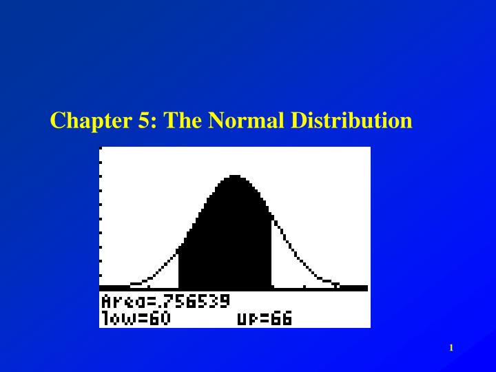
4. Density Curves • The smooth curve drawn over the histogram in the previous example is a density curve. • A mathematical model • Here, we are looking for an overall pattern; we may ignore outliers or slight irregularities. • Area under the curve represents proportions of scores/observations. • The area under a density curve is always 1.0.

5. 15.60 16.10 16.60 17.10 17.60 18.10 18.60 19.10 19.60 We can look at certain areas under the density curve and calculate proportions of observations between certain values.

6. Mean and Median of a Density Curve • Median: Equal-areas point of a density curve • Mean: Balancing point of a density curve • See Figure 5.5, p. 287 • What about the mean and median of a symmetric density curve?

7. Chapter 5: The normal distribution • Begin with Application 5.1B, pp. 291-292

8. Normal Distribution • If we draw a large sample from many populations of interest in science, scores tend to “stack up” in the middle, with a fewer number of scores towards the tails of the distribution. • Many, but certainly not all, distributions can be approximated by a normal density curve. • Normal density curves describe normal distributions.

9. Characteristics of a Normal Curve • Symmetric, single-peaked (uni-modal), and bell-shaped • The exact density curve for a particular normal distribution is described exactly by giving its mean µ and standard deviation σ. • Notation: N(µ , σ) • We can “eye” µ and σ. • See Figure 5.8, p. 290

10. Figure 5.8, p. 290

11. 15.60 16.10 16.60 17.10 17.60 18.10 18.60 19.10 19.60 σ can be found by locating the point of inflection of the density curve.

12. 68-95-99.7 rule (p. 294)

13. Practice Problems • Exercises: • 5.7 and 5.8, p. 297 • Reading through p. 297.

14. Practice Problems • Problems: • 5.9-5.12, p. 297 • 5.13, p. 303

15. What if our score of interest does not fall exactly 1 or 2 or 3 standard deviations from the mean? We need to “standardize.”

16. Standardizing

17. Example Problem • 5.14, p. 303 • Calculate a z-score and use Table A to approximate the answer.

18. Practice Problems • 5.15-5.17, p. 303 • Do by hand first, including a sketch of the problem. • Then, check your answers using the calculator.

19. HW • 5.18, p. 303 • 5.22-5.24, p. 305 • Make sure you have read section 5.1 carefully. • 5.1 Quiz on Friday