Download
1 / 51
520 likes | 598 Views
NETW 703. Network Protocols. BDDs & Theorem Proving Binary Decision Diagrams. Dr. Eng. Amr T. Abdel-Hamid. Lectures are based on slides by: K. Havelund & Agroce , Reliable Software: Testing and Monitoring, CMU. E. Clarke, Formal Methods, to be updated by course name

E N D
NETW703 Network Protocols BDDs & Theorem Proving Binary Decision Diagrams Dr. Eng. Amr T. Abdel-Hamid • Lectures are based on slides by: • K. Havelund & Agroce, Reliable Software: Testing and Monitoring, CMU. • E. Clarke, Formal Methods, to be updated by course name • S. Tahar, E. Cerny and X. Song, “ Formal Verification of Systems”. Winter 2012
Binary Decision Diagrams • Ordered binary decision diagrams (OBDDs) are a canonical form for Boolean formulas. • OBDDs are often substantially more compact than traditional normal forms. • Moreover, they can be manipulated very efficiently. • Introduced at: • R. E. Bryant. Graph-based algorithms for boolean function manipulation. IEEE Transactions on Computers, C-35(8), 1986.
Binary Decision Trees • A Binary decision tree is a rooted, directed tree with two types of vertices, terminal vertices and nonterminal vertices. • Each nonterminal vertex v is labeled by a variable var(v) and has two successors: • low (v) corresponding to the case where the variable is assigned 0, and high (v) corresponding to the case where the variable is assigned 1. • Each terminal vertex v is labeled by value(v) which is either 0 or 1
Example • BDT for a two-bit comparator, f(a1,a2,b1,b2) = (a1 b1) (a2 b2)
Binary Decision Diagram • i.e. exactly like decision TREE
Reduced Ordered BDDs • In practical applications, it is desirable to have a canonical representation for Boolean functions. • This simplifies tasks like checking equivalence of two formulas and deciding if a given formula is satisfiable or not. • Such a representation must guarantee that two Boolean functions are logically equivalent if and • only if they have isomorphic representations.
Reduced Ordered BDD • Canonical Form property • A canonical representation for Boolean functions is desirable: • two Boolean functions are logically equivalent iff they have isomorphic representations • This simplifies checking equivalence of two formulas and deciding if a formula is satisfiable • Two BDDs are isomorphic if there exists a bijection h between the graphs such that • Terminals are mapped to terminals and nonterminals are mapped to nonterminals • For every terminal vertex v, value(v) = value(h(v)), and • For every nonterminal vertex v: var(v) = var(h(v)), h(low(v)) = low(h(v)), and h(high(v)) = high(h(v))
Canonical Form property • Bryant (1986) showed that BDDs are a canonical representation for Boolean functions under two restrictions: • the variables appear in the same order along each path from the root to a terminal • there are no isomorphic subtrees or redundant vertices
Reduced Ordered Binary Decision Diagrams (ROBDDs): CREATION • Canonical Form Property • Requirement (1): Impose total order “<” on the variables in the formula: if vertex u has a nonterminal successor v, then var(u) < var(v) • Requirement (2): repeatedly apply three transformation rules (or implicitly in operations such as disjunction or conjunction)
RoBDD Creation 1) Remove duplicate terminals: eliminate all but one terminal vertex with a given label and redirect all arcs to the eliminated vertices to the remaining one
RoBDD Creation 2. Remove duplicate nonterminals: if nonterminals u and v have var(u) = var(v), low(u) = low(v) and high(u) = high(v), eliminate one of the two vertices and redirect all incoming arcs to the other vertex
3. Remove redundant tests: if nonterminal vertex v has low(v) = high(v), eliminate v and redirect all incoming arcs to low(v)
ROBDD Example • Creating the ROBDD for (x⊕y⊕z)
Canonical Form Property (cont’d) • A canonical form is obtained by applying the transformation rules until no further application is possible • Bryant showed how this can be done by a procedure called Reduce in linear time • Applications: • checking equivalence: verify isomorphism between ROBDDs • non-satisfiability: verify if ROBDD has only one terminal node, labeled by 0 • tautology: verify if ROBDD has only one terminal node, labeled by 1
Variable Ordering Problem • The problem of finding the optimal variable order is NP-complete • Some Boolean functions have exponential size ROBDDs for any order (e.g., multiplier) • Heuristics for Variable Ordering • Heuristics developed for finding a good variable order (if it exists) • Intuition for these heuristics comes from the observation that ROBDDs tend to be smaller when related variables are close together in the order • Variables appearing in a subcircuit are related: they determine the subcircuit’s output should usually be close together in the order • Dynamic Variable Ordering • Useful if no obvious static ordering heuristic applies • During verification operations (e.g., reachability analysis) functions change, hence initial order is not good later on • Good ROBDD packages periodically internally reorder variables to reduce ROBDD size • Basic approach based on neighboring variable exchange • Among a number of trials the best is taken, and the exchange is repeated
Model Checking • The Good: • If it works, model checking (unlike theorem proving) is a push-button tool. • The Bad: • If the system is too large, model checking cannot be applied because of state explosion. • & The Ugly • The system (and/or property) then needs to be suitably “abstracted” in order to use model checking.
Approximate Model Checking • Representing exact state sets may involve large BDDs Compute approximations to reachable states • Potentially smaller representation • Over-approximation : • No bugs found Circuit verified correct • Bugs found may be real or false • Under-approximation : • Bug found Real bug • No bugs found Circuit may still contain bugs Buggy states Reachable states
Theorem Proving • Prove that an implementation satisfies a specification by mathematical reasoning • Implementation and specification expressed as formulas in a formal logic • Required relationship (logical equivalence/logical implication) described as a theorem to be proven within the context of a proof calculus • A proof system: • A set of axioms and inference rules (simplification, rewriting, induction, etc.)
Theorem Proving Idea • Properties specified in a Logical Language (SPEC) • System behavior also in the same language (DES) • Establish (DES -> SPEC) as a theorem. • A logical System: • Alanguage defining constants, functions and predicates • A no. of axioms expressing properties of the constants, function, types, etc. • Inference Rules • A Theorem • `follows' from axioms by application of inference rules has a proof
First-Order Logic • Propositional logic: reasoning about complete sentences. • First-order logic: also reasoning about individual objects and relationships between them. • Syntax • Objects (in FOL) are denoted by expressions called terms: • Constants a, b, c,... ; Variables u, v, w,... ; • f(t1, t2,..., tn) where t1, t2,..., tn are terms and f a function symbol of n arguments • Predicates: • true (T) and false (F) • p(t1, t2,..., tn) where t1, t2,..., tn are terms and p a predicate symbol of n arguments
First-Order Logic (cont.) • Formulas: • Predicates: • P and Q formulas, then P, P Q, P Q, P Q, P Q are formulas • x a variable, P a formula, then x.P, x.Q are formulas (x is not free in P, Q)
First-Order Logic (cont’d) • The Validity Problem of FOL • To decide the validity for formulas of FOL, the truth table method does not work! • Reason: must deal with structures not just truth assignments. • Structures need not be finite ... • Semi-decidable (partially solvable) • There is an algorithm which starts with an input, and • if the input is valid then it terminates after a finite number of steps, and outputs the correct value (Yes or No) • if the input is not valid then it reaches a reject halt or loops forever • Theorem (Church-Turing, 1936) The validity problem for formulas of FOL is undecidable, but semi-decidable. • Some subsets of FOL are decidable.
Higher-Order Logic • First-order logic: only domain variables can be quantified. • Second-order logic: quantification over subsets of variables (i.e., over predicates). • Higher-order logics: quantification over arbitrary predicates and functions. • Higher-Order Logic: • Variables can be functions and predicates, • Functions and predicates can take functions as arguments and return functions as values, • Quantification over functions and predicates. • Since arguments and results of predicates and functions can themselves be predicates or functions, this imparts a first-class status to functions, and allows them to be manipulated just like ordinary values
HOL • Example 1: (mathematical induction) • P. [P(0) (n. P(n) P(n+1))] n.P(n) (Impossible to express it in FOL) • Example 2: Function Rise defined as Rise (c, t) = c(t) c(t+1) • Rise expresses the notion that a signal c rises at time t.
Higher-Order Logic • Advantage: • high expressive power! • Disadvantages: • Incompleteness of a sound proof system for most higher-order logics • Theorem (Gödel, 1931) • “There is no complete deduction system for the second-order logic” • Inconsistencies can arise in higher-order systems if semantics not carefully defined • “Russell Paradox”: • Let P be defined by P(Q) = ¬Q(Q). • By substituting P for Q, leads to P(P) = ¬P(P),
Theorem Proving Systems • Some theorem proving systems: • Boyer-Moore (first-order logic) • HOL (higher-order logic) • PVS (higher-order logic) • Lambda (higher-order logic) From PVS website: “PVS is a large and complex system and it takes a long while to learn to use it effectively. You should be prepared to invest six months to become a moderately skilled user”
HOL • HOL (Higher-Order Logic) developed at University of Cambridge • Interactive environment (in ML, Meta Language) for machine assisted theorem proving in higherorder logic (a proof assistant) • Steps of a proof are implemented by applying inference rules chosen by the user; HOL checks that the steps are safe • All inferences rules are built on top of eight primitive inference rules • Mechanism to carry out backward proofs by applying built-in ML functions called tactics and tacticals • By building complex tactics, the user can customize proof strategies • Numerous applications in software and hardware verification
HOL • HOL provides considerable built-in theorem-proving infrastructure: • a powerful rewriting subsystems • library facility containing useful theories and tools for general use • Decision procedures for tautologies and semi-decision • procedure for linear arithmetic provided as libraries • The approach to mechanizing formal proof used in HOL is due to Robin Milner.
Proof Styles in HOL • Forward proof style: Goal-directed (or Backward) proof style:
Example 1: Logic AND • AND Specification: AND_SPEC (i1,i2,out) := out = i1 ∧ i2 • NAND specification: NAND (i1,i2,out) := out = ¬(i1 ∧ i2) • NOT specification: NOT (i, out) := out = ¬ I • AND Implementation: AND_IMPL (i1,i2,out) := ∃x. NAND (i1,i2,x) ∧ NOT (x,out)
Example 1: Logic AND • Proof Goal: ∀ i1, i2, out. AND_IMPL(i1,i2,out) ⇒ ANDSPEC(i1,i2,out) • Proof (forward) AND_IMP(i1,i2,out) {from above circuit diagram} ∃ x. NAND (i1,i2,x) ∧ NOT (x,out) {by def. of AND impl} NAND (i1,i2,x) ∧ NOT(x,out) {strip off “∃ x.”} NAND (i1,i2,x) {left conjunct of line 3} x =¬ (i1 ∧ i2) {by def. of NAND} NOT (x,out) {right conjunct of line 3} out = ¬ x {by def. of NOT} out = ¬(¬(i1 ∧ i2) {substitution, line 5 into 7} out =(i1 ∧ i2) {simplify, ¬¬ t=t} AND (i1,i2,out) {by def. of AND spec} AND_IMPL (i1,i2,out) ⇒ AND_SPEC (i1,i2,out) Q.E.D.
Inductive Proofs • Inductive Proofs Must Have: • Base Case (value): • where you prove it is true about the base case • Inductive Hypothesis (value): • where you state what will be assume in this proof • Inductive Step (value) • show: • where you state what will be proven below • proof: • where you prove what is stated in the show portion • this proof must use the Inductive Hypothesis sometime during the proof
Example 2 • Prove this statement: • Base Case (n=1): • Inductive Hypothesis (n=p): • Inductive Step (n=p+1): • Show:
Example 3 N-Bit Adder • Verification of Generic Circuits • used in datapath design and verification • idea: verify n-bit circuit then specialize proof for specific value of n, (i.e., once proven for n, a simple instantiation of the theorem for any concrete value, e.g. 32, gets a proven theorem for that instance). • use of induction proof • Specification • N-ADDER_SPEC (n,in1,in2,cin,sum,cout):= (in1 + in2 + cin = 2n+1 * cout + sum)
Example 3 N-Bit Adder • Implementation
Example 3 N-Bit Adder • Recursive Definition: N-ADDER_IMP(n,in1[0..n-1],in2[0..n-1],cin,sum[0..n-1],cout):= ∃ w. N-ADDER_IMP(n-1,in1[0..n-2],in2[0..n-2],cin,sum[0..n-2],w) ∧ N-ADDER_IMP(1,in1[n-1],in2[n-1],w,sum[n-1],cout) Notes: • N-ADDER_IMP(1,in1[i],in2[i],cin,sum[i],cout) = ADDER_IMP(in1[i],in2[i],cin,sum[i],cout) • Data abstraction function (vn: bitvec → nat) to relate bit vectors to natural numbers: • vn(x[0]):= bn(x[0]) • vn(x[0,n]):= 2n * bn(x[n]) + vn(x[0,n-1]
Example 3 N-Bit Adder • Proof goal: ∀ n, in1, in2, cin, sum, cout. N-ADDER_IMP(n,in1[0..n-1],in2[0..n-1],cin,sum[0..n-1],cout) ⇒ N-ADDER_SPEC(n, vn(in1[0..n-1]), vn(in2[0..n-1]), vn(cin), vn(sum[0..n-1]), vn(cout)) • As an example can be instantiated with n = 32: ∀ in1, in2, cin, sum, cout. N-ADDER_IMP(in1[0..31],in2[0..31],cin,sum[0..31],cout) ⇒ N-ADDER_SPEC(vn(in1[0..31]), vn(in2[0..31]), vn(cin), vn(sum[0..31]), vn(cout))
Example 3 N-Bit Adder • Proof by induction over n: • basis step: N-ADDER_IMP(1,in1[0],in2[0],cin,sum[0],cout) ⇒ N-ADDER_SPEC(1,vn(in1[0]),vn(in2[0]),vn(cin),vn(sum[0]),vn(cout)) • Induction Step: [N-ADDER_IMP(n,in1[0..n-1],in2[0..n-1],cin,sum[0..n-1],cout) ⇒ N-ADDER_SPEC(n,vn(in1[0..n-1]),vn(in2[0..n-1]),vn(cin),vn(sum[0..n-1]),vn(cout)) ] ⇒ [N-ADDER_IMP(n+1,in1[0..n],in2[0..n],cin,sum[0..n],cout) ⇒ N-ADDER_SPEC(n+1,vn(in1[0..n]),vn(in2[0..n]),vn(cin),vn(sum[0..n]),vn(cout))]
Conclusions • Advantages of Theorem Proving • High abstraction and expressive notation • Powerful logic and reasoning, e.g., induction • Can exploit hierarchy and regularity, puts user in control • Can be customized with tactics (programs that build larger proofs steps from basic ones) • Useful for specifying and verifying parameterized (generic) datapath-dominated designs • Unrestricted applications (at least theoretically) • Limitations of Theorem Proving: • Interactive (under user guidance): use many lemmas, large numbers of commands • Large human investment to prove small theorems • Usable only by experts: difficult to prove large / hard theorems • Requires deep understanding of the both the design and HOL (while-box verification) • must develop proficiency in proving by working on simple but similar problems.
We are not alone Theorem proving Model checking Testing
Hybrid Verification • Formal Verification using • Theorem Proving + Model Checking Model Checking Theorem Proving
Hybrid Verification ……. G1 G2 G3 Gn G1’’ G2’’ G3’’ Gn’’ |-Goal Imp. Spec. |-Goal Imp.(x y ….) Spec.((y= ..) (…..)) G2’ G3’ G1’ Gn’ Use model checking to verify Sub-Goals
Different Verification Methods • Testing (Simulation/Emulation) • Theorem Proving • Model checking (automatic verification) Testing Theorem Proving Model Checking
Semi-formal Verification Simulation Monitor Simulation Driver Simulation Engine Symbolic Simulation Conventional Diagnosis of Unverified Portions Coverage Analysis Guided vector generation Extension Devadas and Keutzer’s proposal: A pragmatic suggestion for SOC verification
Semi-formal Verification • Smart simulation: • Use properties to generate directed test vectors. • Maximize chances of detecting bugs at small cost • Coverage metrics crucial? • Use metrics to determine • Unexercised parts of design: Guide vector generation • Adequacy of verification: When to stop?
Did you find the BUG yet? • Verification and testing problem is an open question with multi-Billion $ Research per year. • A great Masters Research Topic
A Final Proof • Software engineers want to be real engineers. • Real engineers use mathematics. • Formal methods are the mathematics of software engineering. • Therefore, software engineers should use formal methods. Mike Holloway, NASA