Download
1 / 28
280 likes | 404 Views
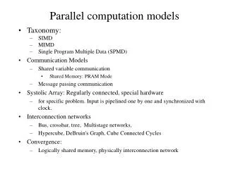
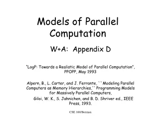
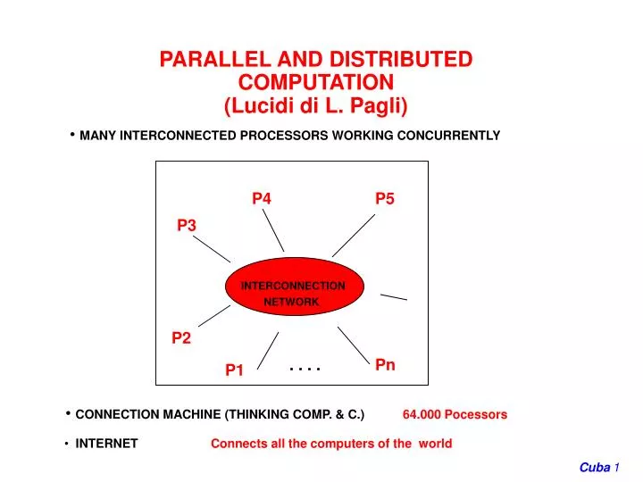
PARALLEL AND DISTRIBUTED COMPUTATION (Lucidi di L. Pagli). MANY INTERCONNECTED PROCESSORS WORKING CONCURRENTLY. P4. P5. P3. INTERCONNECTION. NETWORK. P2. Pn. P1. CONNECTION MACHINE (THINKING COMP. & C.) 64.000 Pocessors.

E N D
PARALLEL AND DISTRIBUTEDCOMPUTATION(Lucidi di L. Pagli) • MANY INTERCONNECTED PROCESSORS WORKING CONCURRENTLY P4 P5 P3 INTERCONNECTION NETWORK P2 . . . . Pn P1 • CONNECTION MACHINE (THINKING COMP. & C.) 64.000 Pocessors • INTERNET Connects all the computers of the world
THREE TYPES OF MULTIPROCESSING FRAMEWORKS, CLOSELY RELATED • CONCURRENT • PARALLEL • PRAM • Bounded-degree network and VLSI • DISTRIBUTED • MULTIPROCESSING ACTVITIES TAKE PLACE IN A SINGLE MACHINE (POSSIBLY USING • SEVERAL PROCESSORS), SHARING MEMORY AND TASKS. • TECHNICAL ASPECTS • PARALLEL COMPUTERS(USUALLY) WORK IN TIGHT SYNCRONY, SHARE MEMORY TO A LARGE EXTENT AND HAVE A VERY FAST AND RELIABLE COMMUNICATION MECHANISM BETWEEN THEM. • DISTRIBUTED COMPUTERSARE MORE INDEPENDENT, COMMUNICATION IS LESS • FREQUENT AND LESS SYNCRONOUS, AND THE COOPERATION IS LIMITED. • PURPOSES • PARALLEL COMPUTERSCOOPERATE TO SOLVE MORE EFFICIENTLY (POSSIBLY) • DIFFICULT PROBLEMS • DISTRIBUTED COMPUTERSHAVE INDIVIDUAL GOALS AND PRIVATE ACTIVITIES. • SOMETIME COMMUNICATIONS WITH OTHER ONES ARE NEEDED. (E. G. DISTRIBUTED DATA BASE OPERATIONS). • PARALLEL COMPUTERS: COOPERATION IN A POSITIVE SENSE • DISTRIBUTED COMPUTERS: COOPERATION IN A NEGATIVE SENSE, ONLY WHEN IT IS NECESSARY
FOR PARALLEL SYSTEMS • WE ARE INTERESTED TO SOLVE ANY PROBLEM IN PARALLEL • FOR DISTRIBUTED SYSTEMS • WE ARE INTERESTED TO SOLVE IN PARALLEL • PARTICULAR PROBLEMS ONLY, TYPICAL EXAMPLES ARE: • COMMUNICATION SERVICES • ROUTING • BROADCASTING • MAINTENANCE OF CONTROL STUCTURE • *SPANNING TREE CONSTRUCTION • TOPOLOGY UPDATE • *LEADER ELECTION • RESOURCE CONTROL ACTIVITIES • LOAD BALANCING • MANAGING GLOBAL DIRECTORIES • * MUTUAL EXCLUSION
PARALLEL ALGORITHMS • WHICH MODEL OF COMPUTATION IS THE BETTER TO USE? • HOW MUCH TIME WE EXPECT TO SAVE USING A PARALLEL ALGORITHM? • HOW TO CONSTRUCT EFFICIENT ALGORITHMS? • MANY CONCEPTS OF THE COMPLEXITY THEORY MUST BE REVISITED • IS THE PARALLELISM A SOLUTION FOR HARD PROBLEMS? • ARE THERE PROBLEMS NOT ADMITTING AN EFFICIENT PARALLEL SOLUTION, • THAT IS INHERENTLY SEQUENTIAL PROBLEMS? • UNDECIDABLE PROBLEMS REMAIN UNDECIDABLE!
PRAM MODEL • Joseph Jajà • An introduction to Parallel Algorithms Addison-Wesley Pub. Comp. 1992 • Karp R.M., Ramachandra V. • A survey of parallel algorithm for shared-memory machines J. Van Leuwen • Ed. Handbook of Theoretical Comp. Science • Jan Parberry • Parallel Complexity Theory Research Notes in Theoretical Computer Science. • John Wiley&Son 1987 • TO FOCUS ON ALGORITHMIC ISSUES INDEPENDENTLY OF PHYSICAL LOCATIONS
1 2 P1 3 P2 Common Memory . ? . . Pi . . Pn m • PRAM n RAM processors numbered from 1 to n and • connected to a common memory of m cells • ASSUMPTION: at each time unit each Pican read a memory cell, make an internal • computation and write another memory cell. • CONSEQUENCE: any pair of processor Pi Pj can communicate in constant time! • Pi writes the message in cell x at time t • Pi reads the message in cell x at time t+1 • Pi
ASSUMPTIONS • Shared-memory: The array A is stored in the global memory and can be accessed by any • processor. • Synchronous mode of operation: In each unit of time, each processor is allowed to execute • an istruction or to stay idle. • There are several variations regarding the handling of simultaneous access to the same • memory location. • EREW-PRAM (exclusive read exclusive write) • CREW-PRAM (concurrent read exclusive write) • CRCW-PRAM (concurrent read CONCURRENT write) and a policy to resolve concurrent writes • Common, Priority, Arbitrary • The three models do not differ substantially in their computationa power! • If each processor can execute its own local program we have a • MIMD (multiple instruction multiple data) model otherwise • SIMD (single instruction multiple data) model
Dal Bertossi Cap. 27 • Sommatoria n log n • Sommatoria n • [R. Grossi]
Important parameters of the efficiency of a parallel algorithm • Tp(n) (or Tp) parallel time • p(n) (or p) number of processors LOWER BOUND of the parallel computation Let A a problem and Ts be the complexity of the optimal sequential (or the best known) algorithm for A, we have: Tp>= Ts/ p Cn = Tp p cost of the parallel algorithm The parallel algorithm can be converted into a sequential algorithm that runs in O(Cn ) time: the single processor simulates the p processorsin p steps for each of the Tpparallel step. If the parallel time would be less than Ts/ p, we could derive a sequential algorithm better than the optimal one!!
Parallel algorithm time1 2 3 processor P1 op1 op2 op3 processor P2 op4 op5 p=2 Tp=3 C=6 can be simulated by a single processor in a number of steps (time) Š 6 Sequential algorithm time1 2 3 4 5 op1 op4 op2 op5 op3 Ts=5 Tp>= Ts/p Ts/Tpspeed up of the parallel algorithm
MAXIMUM on the PRAM • Input: an array A of n=2k elements in the shared memory of a PRAM with n/2 processors • Output: the maximum element stored in location S. • Algorithm MAX • begin • for all kwhere 1 <= k <= log ndo in parallel • if i <= n/2k do in parallel A[i] := max {A[2i], A[2i-1]} • MAX := A[1] • end S P1 A(3) P1 A(3) A(7) P1 P2 A(6) A(7) A(2) A(3) P3 P4 P2 P1 A(2) A(3) A(4) A(5) A(6) A(7) A(8) A(1)
From the previous lower bound and sequential computation C = Tpn not optimal From algorithm MAX C = Tpn = O(nlog n) • Better algorithm: • divide the n elements in k =n/log n subsets of log n elements each P1 P2 P3 Pk ................... m1 m2 m3 mk • each processor computes the maximum mi of its subsets • with the sequential algorithm in time O(log n) • algorithm MAX is executed among the local maxima, time • O(log (n/log n)) = O(logn - loglog n)= O(logn) Overal time: Tp = O(log n) and p= n/ log n optimal C = Tpn = O(n)
PERFORMANCE OF PARALLEL ALGORITHM Four ways of measuring the performance of parallel algorithm: 1. P(n) processors and Tp(n) time. 2. C(n) = P(n)Tp(n) cost and Tp(n) time. The number of processors depends on the size n of the problems. The second relation can be generalized to any number p<P(n) processors each of the Tp parallel step can be simulated by the p processors in O(P(n)/p) substeps; this simulation takes a total of O(Tp(n)P(n)/p) time. 3. O(Tp(n)P(n)/p) time for any number p<P(n) processors If the number of processors p is larger than P(n), we can clearly achieve the runnng time Tp(n) by using P(n) processors only. Relation 3 can be further generalized. 4. O(C(n)/p + Tp(n)) time for any number p processors In conclusion,in the design of a PRAM alg., we can assume as many processor we need and use the proper relation to analyze it.
PERFORMANCE OF ALGORITHM MAX 1. P(n)= n/2 processors and Tp(n) =O(log n) time. 2. C(n) = P(n)Tp(n) = O(n log n) cost and Tp(n)= O(log n) time Assume p= log n processors 3. O(Tp(n)P(n)/p) = O (logn n/logn) = O(n) time Therefore 4. O(logn n/p + logn) time. If p<=n, O(log n)time, otherwise O(logn n/p ) time. Work W(n) of a parallel algorithm: total number of operations used. Work of alg. MAX: W(n) = SUMj=1, logn(n/2j) + 1 = O(n) W(n) < C(n) W(n) measures the total number of operations and has nothing to do with the number of processors available, while C(n) measures the cost of the alg. relative to the number p of processors available.
Work-time presentation of a parallel algorithm any number of parallel operations at each time unit is allowed BRENT PRINCIPLE : given a parallel algorithm that runs in time T(n) and requires W(n) work, we can adapt this algorithm to run on a p-processors PRAM in time Tp(n) < |W(n)/p| + T(n) Let Wi(n) be the number of operation of time unit i, 1<= i <= T(n). Simulate each set of Wi(n) operations in |Wi(n)/p| parallel steps of the p processors, for each 1<= i <= T(n). The p-processors PRAM algorithm takes <=SUMi |Wi(n)/p| <=SUMi (|Wi(n)/p| +1) <SUMi |Wi(n)/p| + T(n). The Brent Principle assumes that the scheduling of the operations to the processors is always a trivial task. This is not always true. It’s easy if we use C(n) in place of W(n)
t 1 7 14 17 25 30 algorithm A1 2 8 15 18 3 9 16 19 T1 = 6 4 10 20 5 11 21 29 6 12 22 13 23 36 24 W(n) =36 Wi 6 7 3 8 5 7 A1 can be simulated by A2 with 3 processors in timeT2(n) <= 36/3 + 6 =18 1 4 7 10 13 14 17 20 23 25 28 30 33 36 2 5 8 11 15 18 21 24 26 29 31 34 T2 = 14 3 6 9 12 16 19 22 27 32 35 t1 t2 t3 t4 t5 t6
Dal Bertossi cap. 27 • Tecniche di base: • Somme prefisse • Ordinamento non ottimo • List ranking con pointer jumping • Ciclo euleriano • [R. Grossi]
PARALLEL DIVIDE AND CONQUER • Partion the input in several subsets of almost equal size • Solve recursively the subproblem defined by each subset • Combine the solutions of the subproblems into a solution • to the overall problem CONVEX HULL sequential algorithm O(n logn) v3 v4 v2 UPPER HULL v1 v5 LOWER HULL v7 v6 p q • Sort the x-coordinates in increasing order • Compute the UPPER HULL Tp =O(log n)
w. l. o. g., let x (v1) < x (v2) < . . .< x (vn) n = 2k • Divide the points in two subsets S1 (v1, v2 , . . .,vn/2) S2 (vn/2+1, . . .,vn) suppose the UPPER HULL of S1 and S2 is already computed q2 b a q’2 q3 q’3 Compute ab : upper common tangent q’4 q4 q1 q’1 S1 q5 S2 • The UPPER HULL of S is formed by q1 , . . . , qi = a, q’j = b, . . . ,q’s Algorithm UPPER HULL (Sketch) 1. if n<=4 use brute force method to determine UH(S) 2. Let S1 (v1, v2 , . . .,vn/2), S2 (vn/2+1, . . .,vn) recursively compute UH(S1) and UH(S2) in parallel (Tp(n/2) time and 2W(n /2) operations) 3. Find the Upper Common Tangent between UH(S1) and UH(S2) and deduce UH(S) O(log n sequential time) O(n ) operations Tp(n) = Tp(n/2) +O(log n)= O(log2 n) W(n) = O(nlogn)
Intractable problems remain intractable in parallel For an intractable problem (NP-hard) the only known solution require exponential time: Ts = abn p = nc (polynomial in the size of the input) From the lower bound: TP>= abn/ n c > a(b/2)n for large value of n still exponential We consider only the classP, and in particular the class NCÎ P. NC is the class of all (decision) problems that can be solved in solved in polylog parallel time (i. e. Tp is of order O(logkn)), with a polynomial number of processors. NC contains problems that can be efficiently solved in parallel
PARALLEL SEQUENTIAL Class NC Class P Efficient Algorithm Efficient Algorithm ? ? NC = P P = NP • There are problems belonging to P for • which NO EFFICIENT PARALLEL • algorithm is known. • There is no proof that such an algorithm not • exists P-complete Problems NP-complete Problems Monotone Circuit Value Satisfiability P NP NP1 P1 MCV SAT P2 NP2 . P3 . NP3 . . Ph NPK Goldshlager Th. (1984) Cook’s Th. (1969)
MONOTONE CIRCUIT VALUE PROBLEM (MCVP) a b c d e f g z =(((a AND b) OR c) AND d) AND ((e AND f) OR g) z Determine the value of the single output of a Boolean Circuit consisting of two-valued AND and OR gates and a set of inputs and their complements, DEPTH FIRST SEARCH dfs numbers 1 a 1 b 2 c 5 d 3 e 4 f 6 g 7 a b 2 2 1 1 3 e c d 1 2 2 3 f g arcs numbered according to the order of appereance on the adjacency list
MAX FLOW 3 5 4 4 2 2 2 2 1 1 0 1 1 1 1 1 1 1 s t s t 1 2 0 2 3 3 1 1 3 3 f = 6 A directed graph N (network) with two distinguished vertices: source s and sink t; each arc is labelled with its capacity (positive integer). A flow f is a function, such that 1. 0 <= f(e) <= c(e), for all arcs e (capacity constraint) 2. the sum of the flow of all incoming arcs to any node (!= s,t), is equal to sum of the flow on all outgoing arcs. (conservation constraint) The value of the FLOW is given by the sum of the flow of the outgoing arcs of s (= to the sum of the flow of all incoming arcs to t). Findthe maximum possible value of the flow. Sequential Algorithm O(n3) No efficient parallel solution is known
Decisional Parallel Problems Reducibility Notion: Let A1 and A2 be decisional problems. A1 is NC-reducible to A2 if there exists an NC-algorithm that transforms an arbitrary input u1 of A1 into an input u2 of A2, such that A1 answer yes for u1 if and only if A2 answer yes for u2. A2 is at least as difficult as A1 A problem A is P-Complete if every problem in the class P is NC-reducible to A If A is P-complete If A is NP-complete AÎNC iff P=NC AÎP iff P=NP The hope of finding an efficient parallel algorithm is very low • To show that a problem A is P-Complete • - AÎ P • - MCVP is NC-reducible to A MCVP input: Acyclic network of gates AND, OR (two-valued input) and an assignement of constant values 0,1 at each input line output: compute the value of the single output value
Sketch of the GOLDSHLAGER’S theorem • An arbitrary problem AÎ P can be formulated as an MCVP problem. • MCVP Î P because z can be computed in O(n) sequential time. • if A Î P is accepted by a deterministic TM in time T(n), polynomial for any input n. • output • 1 n 0 input Q = {q1, . . . , qs} set of States å = { a1, . . . , am} tape’s alphabet d : Q x å Q x å x { L, R} transition function The corresponding boolean circuit is defined by the following boolean functions: 1. H (i,t) = 1 if the head is on cell i a time t. 0 <= T <= T(n), 1<= i <= T(n). 2. C(i, j, t) = 1 if the cell i contains the symbol aj at time t.0 <= T<= T(n), 1<= i <=T(n), 1<= j <= m. 3. S (k,t) =1 if the state of the TM is qkat time t. 1<=k<= s, 0<= T<= T(n). Each step of the Turing machine can be described by one level of the circuit computing H (i, t), C( i, j, t) and S(k, t ).
0 1 EX: q1 1q2R - TM q2 0q3R 1q2L Q = {q1, q2, q3} S = {0,1} q3 0q3L 1q3R 1 1 t = 0 1 , i = 1 1 , i = 1, j =2 1, k= 1 H (i, 0) C (i, j, 0) S (k, 0) = 0 , 2 < i < n 0 , i = 1, j =2 0, k°1 i-1 i i+1 t > 0 H (i, t) = ( H (i-1, t-1) AND “right shift”) OR ( H(i+1, t-1) AND “left shift”) “left shift” =((S (2, t-1) AND C (i+1, 2, t-1)) OR (S(3, t-1) AND C (i+1, 1, t-1)) analogously compute C (i, j, t) and S (k, t). The circuit value is given by C(1, * , T (n)) and can be computed in O (log n) time with a quadratic number of processors.
THE PRAM IS A THEORETICAL (UNFEASIBLE) MODEL • The interconnection network between processors and memory would require • a very large amount of area . • The message-routing on the interconnection network would require time • proportional to network size (i. e. the assumption of a constant access time • to the memory is not realistic). WHY THE PRAM IS A REFERENCE MODEL? • Algorithm’s designers can forget the communication problems and focus their • attention on the parallel computation only. • There exist algorithms simulating any PRAM algorithm on bounded degree • networks. • E. G. A PRAM algorithm requiring time T(n), can be simulated in a mesh of tree • in time T(n)log2n/loglogn, that is each step can be simulated with a slow-down • of log2n/loglogn. • Instead of design ad hoc algorithms for bounded degree networks, design more • general algorithms for the PRAM model and simulate them on a feasible network.
For the PRAM model there exists a well developed body of techniques • and methods to handle different classes of computational problems. • The discussion on parallel model of computation is still HOT • The actual trend: • COARSE-GRAINED MODELS (BSP, LOGP) • The degree of parallelism allowed is independent from the number • of processors. • The computation is divided in supersteps, each one includes • local computation • communication phase • syncronization phase the study is still at the beginning!