Download
1 / 29
300 likes | 609 Views
Lossless Compression(2). Hongli Luo. Lecture 4: Lossless Compression(2). Topics Huffman coding Arithmetic encoding Dictionary-based Coding (LZW algorithm) Lossless image compression. Huffman Coding. Huffman Coding Algorithm - a bottom-up approach

E N D
Lossless Compression(2) Hongli Luo
Lecture 4: Lossless Compression(2) • Topics • Huffman coding • Arithmetic encoding • Dictionary-based Coding (LZW algorithm) • Lossless image compression
Huffman Coding • Huffman Coding Algorithm - a bottom-up approach 1. Initialization: Put all symbols on a list sorted according to their frequency counts. 2. Repeat until the list has only one symbol left:: (1) From the list pick two symbols with the lowest frequency counts. Form a Huffman subtree that has these two symbols as child nodes and create a parent node. (2) Assign the sum of the children's frequency counts to the parent and insert it into the list such that the order is maintained. (3) Delete the children from the list. 3. Assign a codeword for each leaf based on the path from the root.
Huffman Coding In Fig. 7.5, new symbols P1, P2, P3 are created to refer to the parent nodes in the Huffman coding tree. The contents in the list are illustrated below: • After initialization: L H E O • After iteration (a): L P1 H • After iteration (b): L P2 • After iteration (c): P3
Properties of Huffman Coding • Unique Prefix Property: No Huffman code is a prefix of any other Huffman code - precludes any ambiguity in decoding. • Optimality: minimum redundancy code - proved optimal for a given data model (i.e., a given, accurate, probability distribution): • The two least frequent symbols will have the same length for their Huffman codes, differing only at the last bit. • Symbols that occur more frequently will have shorter Huffman codes than symbols that occur less frequently. • The average code length for an information source S is strictly less than + 1. Combined with Eq. (7.5), we have:
Properties of Huffman Coding • Decoding for the Shannon-Fano and Huffman coding is trivial if the coding table is sent before the data • There is a bit of an overhead for sending this • But negligible if the data file is big • Entropy in the above example: H = (2 * 1.32 + 1 * 2.32 + 1 * 2.32 + 1 * 2.32) / 5 = 9.6 / 5 = 1.92 number of bits needed for Huffman Coding is: = 10/5 = 2 • Huffman coding is used in Fax, JPEG and MPEG
Extended Huffman Coding • Motivation: All codewords in Huffman coding have integer bit lengths. It is wasteful when pi is very large. • Why not group several symbols together and assign a single codeword to the group as a whole? • Extended Alphabet: For alphabet S = (s1, s2, … sn}, if k symbols are grouped together, then the extended alphabet is: • the size of the new alphabet S(k) is nk.
Extended Huffman Coding (cont'd) • It can be proven that the average # of bits for each symbol is: • An improvement over the original Huffman coding, but not much. • Problem: If k is relatively large (e.g., k >= 3), then for most practical applications where n >> 1, nkimplies a huge symbol table - impractical.
Adaptive Huffman Coding • Adaptive Huffman Coding: statistics are gathered and updated dynamically as the data stream arrives.
Adaptive Huffman Coding (Cont'd) • Initial_code assigns symbols with some initially agreed upon codes, without any prior knowledge of the frequency counts. • update_tree constructs an Adaptive Huffman tree. It basically does two things: • increments the frequency counts for the symbols (including any new ones). • updates the configuration of the tree. • The encoder and decoder must use exactly the same initial_code and update_tree routines. • For “AADCCDD”, “0000011000100000011001101101” is sent • It is important to emphasize that the code for a particular symbol changes during the adaptive Huffman coding process. • For example, after AADCCDD, when the character D overtakes A as the most frequent symbol, its code changes from 101 to 0.
Table 7.4 Sequence of codes sent to the decoder Symbol Codes NEW 0 A 00001 A 1 NEW 0 D 00100 NEW 0 C 00011 C 001 D 101 D 101
Arithmetic Coding • Arithmetic coding is a more modern coding method that usually out-performs Huffman coding. • Initial idea was introduced by Shannon in 1948. • Huffman coding assigns each symbol a codeword which has an integral bit length. Arithmetic coding can treat the whole message as one unit. • Known to outperform Huffman coding. • A message is represented by a half-open interval [a, b) where a and b are real numbers between 0 and 1. • Initially, the interval is [0,1). • When the message becomes longer, the length of the interval shortens and the number of bits needed to represent the interval increases. • In practice, the input data is usually broken into chunks.
Arithmetic Coding • Fractions in Binary 0.1 binary = 2-1 decimal = 0.5 decimal 0.01 binary = 2-2 decimal = 0.25 decimal 0.11 binary = 2-1 + 2 -2 decimal = 0.75 decimal • For “CAEE$”, generate a binary fraction between [0.33184, 0.33220) • the binary fraction number obtained using arithmetic coding is 0.01010101, which is 0.33203125 in decimal fraction. binary 0.01010101 decimal 0.33203125 = (2)-2+ (2)-4 + (2)-6 + (2)-8 binary 0.01010110 decimal 0.3333984375 binary 0.01010100 decimal 0.328125 • Therefore, to encode the sequence of symbol “CAEE$”, 8 bits are needed.
Arithmetic Coding • PROCEDURE 7.2 Generating Codeword for Encoder BEGIN code = 0; k = 1; while (value(code) < low) { assign 1 to the kth binary fraction bit if (value(code) > high) replace the kth bit by 0 k = k + 1; } END • The final step in Arithmetic encoding generates a number (a binary fraction) that falls within the range [low; high). • The above algorithm will ensure that the shortest binary codeword is found.
Arithmetic Coding • The arithmetic coding algorithm needs to use very high-precision numbers to do encoding when the interval shrinks. This adds to the implementation difficulty. • It is possible to rescale the intervals and use only integer arithmetic for a practical implementation. • Known to outperform Huffman coding e.g., for symbols {y,u,v}, p(y) = 0.5, p(u)=0.4, p(v) = 0.1 To encode “uuu”, huffman coding needs 6 bits, e.g., “101010”, arithmetic coding needs 4 bits. 0.1101binary (0.8125 decimal).
Dictionary-based Coding • Question : How to encode the Oxford Concise English dictionary which contains about 159,000 entries? • Solution: • Encode each word as 18 bit number • too many bits per word, a dictionary is needed. • Build the dictionary adaptively (LZW) • Only the initial dictionary needs to be transmitted • The decoder is able to build the rest of the dictionary from the encoded sequence
Dictionary-based Coding • LZW uses fixed-length codewords to represent variable-length strings of symbols/characters that commonly occur together, • e.g., words in English text. • the LZW encoder and decoder build up the same dictionary dynamically while receiving the data. • LZW places longer and longer repeated entries into a dictionary, and then emits the code for an element, rather than the string itself, if the element has already been placed in the dictionary. • Used in GIF files, Adobe PDF file, UNIX compress Utility (LZ only), gzip, gunzip, Windows WinZip, GIF and TIFF compression.
Lossless Image Compression • Approaches of Differential Coding of Images: • Use the idea that neighboring image pixels are similar • Given an original image I(x, y), using a simple difference operator we can define a difference image d(x, y) as follows: d(x, y) = I(x, y) − I(x − 1, y) (7:9) or use the discrete version of the 2-D Laplacian operator to define a difference image d(x,y) as d(x, y) = 4I(x, y) − I(x, y − 1) − I(x, y +1)−I(x+1, y)−I(x−1, y) (7.10) • Usually the entropy of the original image is larger than the entropy of the differential image, so we can apply VLC (such as Huffman coding) to the differential image and achieve better compression ratio.
Fig. 7.9: Distributions for Original versus Derivative Images. (a,b): Original gray-level image and its partial derivative image; (c,d): Histograms for original and derivative images.
Example, • Encoding using d(x,y) = I(x,y) – I(x-1,y) The original image Differential image • Decoding using I(x,y) = I(x-1,y) + d(x,y) • Differential image The reconstructed image
Lossless JPEG • Lossless JPEG: A special case of the JPEG image compression. • The Predictive method 1. Forming a differential prediction: A predictor combines the values of up to three neighboring pixels as the predicted value for the current pixel, indicated by `X' in Fig. 7.10. The predictor can use any one of the seven schemes listed in Table 7.6. 2. Encoding: The encoder compares the prediction with the actual pixel value at the position `X' and encodes the difference using one of the lossless compression techniques we have discussed, e.g., the Huffman coding scheme.
Predictors that use only 1 pixel are called first-order. • Predictors that use 2, 3 or more pixels are called second-order, third order or high-order. Example: If use P = A/2 + B/2 Then d(x,y) = X – P = I(x,y) – P d(x,y) = I(x,y) – (I(x-1,y)/2 + I(x,y-1)/2)