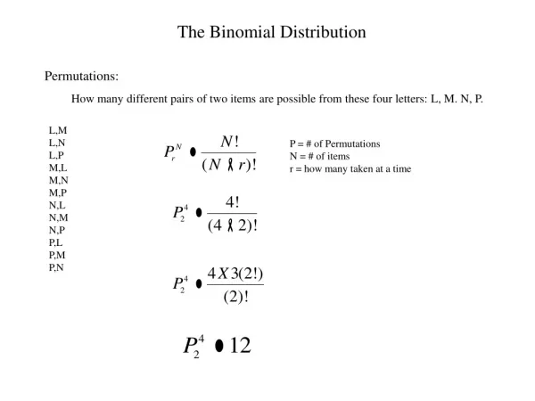
Download
1 / 20
660 likes | 2.37k Views
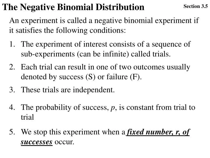
The Negative Binomial Distribution. Section 3.5. An experiment is called a negative binomial experiment if it satisfies the following conditions:. The experiment of interest consists of a sequence of sub-experiments (can be infinite) called trials.

E N D
The Negative Binomial Distribution Section 3.5 An experiment is called a negative binomial experiment if it satisfies the following conditions: The experiment of interest consists of a sequence of sub-experiments (can be infinite) called trials. Each trial can result in one of two outcomes usually denoted by success (S) or failure (F). These trials are independent. The probability of success, p, is constant from trial to trial We stop this experiment when a fixed number, r, of successes occur.
The Negative Binomial Distribution Section 3.5 What the above is saying: The experiment consists of a group of independent Bernoulli sub-experiments, where r (not n), the number of successes we are looking to observe, is fixed in advance of the experiment and the probability of a success is p. What we are interested in studying is the number of failures that precede the rth success. Called negative binomial because instead of fixing the number of trials n we fix the number of successes r.
The Negative Binomial Distribution Section 3.5 Example: Observe the light-bulb production line testing each bulb, and stopping the production process for maintenance after the 3rd observed defective (S). From experience, the probability that a light bulb is defective is 0.1.
The Negative Binomial Distribution Section 3.5 Identify the experiment of interest and understand it well (including the associated population) The experiment consists of a sequence of independent Bernoulli sub-experiments, where r = 3, the number of successes we are looking to observe, is fixed in advance of the experiment and the probability of a success is p = 0.1. So the experiment qualifies as a negative binomial experiment.
The Negative Binomial Distribution Section 3.5 Identify the sample space (all possible outcomes) S = {SSS, FSSS, SFSS, SSFS, FFSSS, …, FFFSSS …} How many? Still discrete?
The Negative Binomial Distribution Section 3.5 Identify an appropriate random variable that reflects what you are studying (and simple events based on this random variable) X = # of failures until the 3rd success Snew= {0, 1, 2, …}
The Negative Binomial Distribution Section 3.5 Construct the probability distribution associated with the simple events based on the random variable X = 0, how many simple events in association? Probability is? X = 1, how many associated simple events (outcomes)? The probability is? X = 2, how many associated simple events (outcomes)? The probability is? The general equation describing this distribution is?
The Negative Binomial Distribution Section 3.5 The resulting distribution in table format:
The Negative Binomial Distribution Section 3.5 The resulting distribution in table format:
The Negative Binomial Distribution Section 3.5 Notation in association with the negative binomial experiment: The negative binomial random variable X = the number of failures (F’s) until the rth success. We say X is distributed negative Binomial with parameters r and p,
The Negative Binomial Distribution Section 3.5 pmf is: CDF is
The Negative Binomial Distribution Section 3.5 Mean Variance Standard deviation
The Negative Binomial Distribution Section 3.5 Mean Variance Standard deviation
The Negative Binomial Distribution Section 3.5 What is the chance that you will observe 3 defective light bulbs after observing 27 +/- 2*16.43 (-5.86, 59.86) failures? Approximately using Chebyshev’s rule: Exactly from using R:
The Negative Binomial Distribution Section 3.5 A special case of the negative binomial is when r = 1, then we call the distribution geometric. Notation in association with the geometric experiment: The geometric random variable X = the number of failures (F’s) until the 1stsuccess. We say X is distributed geometric with parameter p,
The Negative Binomial Distribution Section 3.5 pmf is: CDF is
The Negative Binomial Distribution Section 3.5 Mean Variance Standard deviation
The Negative Binomial Distribution Section 3.5 Example: Observe the light-bulb production line testing each bulb, and stopping the production process for maintenance after the 1st observed defective (S). From experience, the probability that a light bulb is defective is 0.1. Now we can start to jump in and solve problems directly as we have the base! (I hope). This experiment looks like a geometric one. So the distribution that we can use to find probabilities is:
The Negative Binomial Distribution Section 3.5 P(X > 3) = ? Mean is? What does it mean? Variance and standard deviation are? Chance of being within two standard deviations from the mean? Exact and Chebyshev!
The Poisson distribution Section 3.6 Moving away from the solid Bernoulli based trials to approximate distributions.