Adaline Schematic

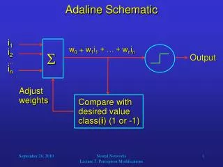
1. Adaline Schematic i1 • Adjust weights w0 + w1i1 + … + wnin i2  Output … in Compare with desired valueclass(i) (1 or -1) Neural Networks Lecture 7: Perceptron Modifications

2. The Adaline Learning Algorithm • The Adaline uses gradient descent to determine the weight vector that leads to minimal error. • Error is defined as the MSE between the neuron’s net input netj and its desired output dj (= class(ij)) across all training samples ij. • The idea is to pick samples in random order and perform (slow) gradient descent in their individual error functions. • This technique allows incremental learning, i.e., refining of the weights as more training samples are added. Neural Networks Lecture 7: Perceptron Modifications

3. The Adaline Learning Algorithm • The Adaline uses gradient descent to determine the weight vector that leads to minimal error. Neural Networks Lecture 7: Perceptron Modifications

4. The Adaline Learning Algorithm • The gradient is then given by For gradient descent, w should be a negative multiple of the gradient: Neural Networks Lecture 7: Perceptron Modifications

5. The Widrow-Hoff Delta Rule • In the original learning rule Longer input vectors result in greater weight changes, which can cause problems if there are extreme differences in vector length in the training set. Widrow and Hoff (1960) suggested the following modification of the learning rule: Neural Networks Lecture 7: Perceptron Modifications

6. Multiclass Discrimination • Often, our classification problems involve more than two classes. • For example, character recognition requires at least 26 different classes. • We can perform such tasks using layers of perceptrons or Adalines. Neural Networks Lecture 7: Perceptron Modifications

7. Multiclass Discrimination w11 o1 w12 i1 • A four-node perceptron for a four-class problem in n-dimensional input space o2 i2 . . o3 . in o4 w4n Neural Networks Lecture 7: Perceptron Modifications

8. Multiclass Discrimination • Each perceptron learns to recognize one particular class, i.e., output 1 if the input is in that class, and 0 otherwise. • The units can be trained separately and in parallel. • In production mode, the network decides that its current input is in the k-th class if and only if ok = 1, and for all j  k, oj = 0, otherwise it is misclassified. • For units with real-valued output, the neuron with maximal output can be picked to indicate the class of the input. • This maximum should be significantly greater than all other outputs, otherwise the input is misclassified. Neural Networks Lecture 7: Perceptron Modifications

9. Multilayer Networks • Although single-layer perceptron networks can distinguish between any number of classes, they still require linear separability of inputs. • To overcome this serious limitation, we can use multiple layers of neurons. • Rosenblatt first suggested this idea in 1961, but he used perceptrons. • However, their non-differentiable output function led to an inefficient and weak learning algorithm. • The idea that eventually led to a breakthrough was the use of continuous output functions and gradient descent. Neural Networks Lecture 7: Perceptron Modifications

10. Multilayer Networks • The resulting backpropagation algorithm was popularized by Rumelhart, Hinton, and Williams (1986). • This algorithm solved the “credit assignment” problem, i.e., crediting or blaming individual neurons across layers for particular outputs. • The error at the output layer is propagated backwards to units at lower layers, so that the weights of all neurons can be adapted appropriately. • The gradient descent technique is similar to the Adaline, but propagating the error requires some additional computations. Neural Networks Lecture 7: Perceptron Modifications

11. Terminology output vector o1 o2 • Example: Network function f: R3  R2 output layer hidden layer input layer x1 x2 x3 input vector Neural Networks Lecture 7: Perceptron Modifications