Download
1 / 50
500 likes | 612 Views
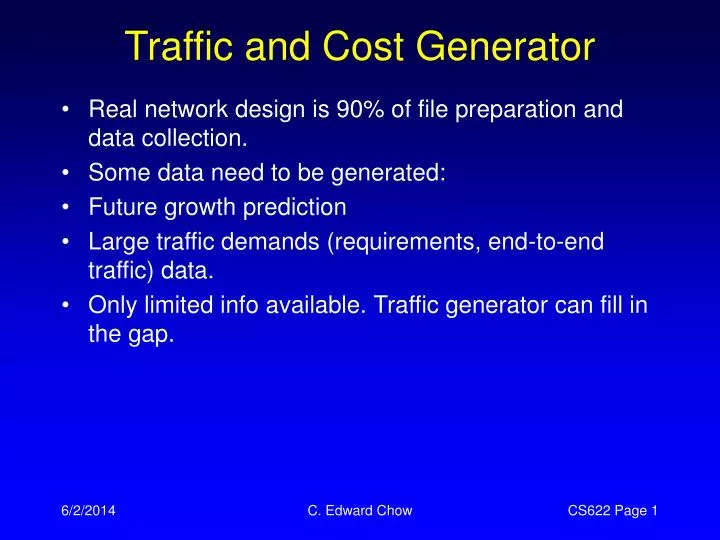
Traffic and Cost Generator. Real network design is 90% of file preparation and data collection. Some data need to be generated: Future growth prediction Large traffic demands (requirements, end-to-end traffic) data. Only limited info available. Traffic generator can fill in the gap.

E N D
Traffic and Cost Generator • Real network design is 90% of file preparation and data collection. • Some data need to be generated: • Future growth prediction • Large traffic demands (requirements, end-to-end traffic) data. • Only limited info available. Traffic generator can fill in the gap. C. Edward Chow
Delite Network File Format Goal: simple extensible. C. Edward Chow
Tariff, Equipment, Param Format C. Edward Chow
Cluster Site Notation • Here the PARENT column deal with the homing of this site. C. Edward Chow
Sites Population and Level C. Edward Chow
Traffic Units for Various Networks C. Edward Chow
Traffic Generation • Assume Uniform Traffic. Traf(i,j)=C. Traffic from node i to node j is C. • Assume Random Traffic . Traf(i,j) is some distribution between a minimum and a maximum value.What distribution is the following code generated? C. Edward Chow
Random Mux Circuit Traffic Generation • D56 56kbps links • Nreq circuits will be generated. C. Edward Chow
More Realistic TrafficFormula 1 C. Edward Chow
Add Offset and Scale Factor • A is scale factor • Population offset (say 0.05) avoid zeros; • Distance Offset. C. Edward Chow
Traffic Normalization • Example 4.1: 50 sites linked by 85 E1 lines. The average of hops is 2.75 and the links have an average utilization of 0.55. What value of a should be chosen to generate the traffic? • Solution: • Total carried traffic on the network = • Let T= • We choose a =69,632,000/T C. Edward Chow
Row Normalization • With row indicating source, column indicating destination in the traffic matrix. • The traffic from node i to other nodes is • We can then define • This allows us to match the synthetic traffic to the observed traffic. C. Edward Chow
Row and Column Normalization C. Edward Chow
Example: 5 node network • Site data and observed Traffic in and out of a node. C. Edward Chow
1st round with Pop_Power=1 and Dist_Power=1 C. Edward Chow
1st round Row and Column Scale Factors and Modified Traffic C. Edward Chow
2nd Round Traffic Matrix C. Edward Chow
2nd Round Row and Column Scale Factors • Scale =1.009 C. Edward Chow
5 Iteration later C. Edward Chow
Considering Level (Traffic Type of Nodes) • Level Matrix (uneven traffic btw Level 1 and Level 2) • Formula C. Edward Chow
Final Traffic Formula • Consider the random traffic, 0<=rf: random fraction<=1 C. Edward Chow
Traffic Generators and Sensitivity Analysis • Often useful to generate traffic suites than a single set of traffic. • It can be used to study how network responds to change. • Sometimes, there is a requirement that network not be re-designed for a period of time. C. Edward Chow
A Case Study: “Green Field” Redesign of a Network • Green field mean “unconstrained to reuse the network already in place. • 7 nodes in Squareworld. • Distance Matrix: C. Edward Chow
Parameter for Terminal Traffic • N1-N5 each has 100 users, N6-N7 each has 200 users. Level one has 600 users. C. Edward Chow
Modeling User Session • Traffic Matrix (by observing control point data) • Here N4 and N7 have host computers. C. Edward Chow
Voice vs. Email Cost • Fixed cost of email vs. time dependent cost of voice C. Edward Chow
Internal Email Traffic Parameter • Total population=900. • 8 2000bytes email in busy hour. • Why only normalize on ROW? C. Edward Chow
Internal Email Traffic Matrix • Generated by Traffic generator using the parameters in previous page. Note that the total email traffic includes those that send to destination in the same site. C. Edward Chow
Internal Email Actual Traffic • Remove the diagonal entries leave the inter-site traffic. C. Edward Chow
Internal Web Page Traffic • 25% web fetches are internal. • 23 pages/hour/user • Each page access results 5 128Byte datagrams outbound and 5 128 Byte datagrams inbound, 3500 byte HTML and related files inbound. • Outbound traffic/user=0.25*23*5*128*8/3600=8.177bps • Inbound traffic/user=8.177+0.25*23*3500*8/3600=52.9bps. • TRAFIN and TRAFOUT only consider traffic initiated from the site. C. Edward Chow
Internal Web Page Traffic Parameter • The sum of row traffic = TRAFOUT C. Edward Chow
Internal Web Page Traffic Out • 92*4+180*2=730? Vs 818 This is due to 818*(1/9)=92 of the traffic is intra-site.The other 818*(8/9)=727 is the actual TRAFOUT that spread to all other 6 nodes. • 183*5+362=1277? Vs 1636 due to Arbitrary Dist_offset? C. Edward Chow
Internal Web Page Traffic Inbound • The ratio between the inbound traffic and outbound traffic = 52.90/8.177=6.46875. • The inbound traffic matrix=6.46875* Ttrwhere Ttr is the transpose of matrix T. C. Edward Chow
External Web Page Traffic • 75% of web traffic to external sites. • 23 pages/hour/user • Each page access results 5 128Byte datagrams outbound and 5 128 Byte datagrams inbound, 3500 byte HTML and related files inbound. • Outbound traffic/user=0.75*23*5*128*8/3600=24.533bps • Inbound traffic/user=24.533+0.75*23*3500*8/3600=158.70bps. • Typo in text: “8.17 plus” should be “24.533 plus” C. Edward Chow
Partition DB Site Traffic • Total DB=200GB, 80 GB at N1, 60 GB at N4, 60GB at N7. • 900 users. Per user has 15 queries/hour, 300B request(out), 4000B data(in). 3 updates/hour, 8000B(out), 1000B(in). • Query traffic to server: 15*300*8/3600=10bps. • Query traffic from server: 15*4000*8/3600=133.333bps. • Update traffic to server: 3*8000*8/3600=53.333bps. • Update traffic from server: 3*1000*8/3600=6.666 bps. 100*(10+53.33)=6333100*(133.3+6.6)=14000 63.33*900*0.4=22,799 140*900*0.4=50,400 N1 has 80GB, 40% of Total DB. C. Edward Chow
Partition DB Traffic Inbound • 40% of N2 6333 outbound DB traffic go to N1=0.4*6333=2533. • 0.3*6333=1900 to N4 and 1900 to N7. C. Edward Chow
Partition DB Traffic Outbound • The ratio between the inbound traffic and outbound traffic = 14000/6333. • The inbound traffic matrix=14000/6333* Ttrwhere Ttr is the transpose of matrix T. C. Edward Chow
Replicated DB Client-Server Query • DB are replicated at site N1, N4, and N7. • Assume static allocation of clients to servers.N5N1, N3N4, N2,N6N7. • N5 has 100 pop*10bps/pop=1000 bps query outbound; 100*133.33=13,333 bps query inbound. C. Edward Chow
Replicated DB Client-Server Update • DB are replicated at site N1, N4, and N7. • Assume static allocation of clients to servers.N5N1, N3N4, N2,N6N7. • N5 has 100 pop*53 1/3 bps/pop=5333 bps update outbound; 100*6 2/3=666 bps update inbound. C. Edward Chow
Replicated DB Update Server-Server • Same 53 1/3 bps update request per user and 6 2/3 bps update response per user. • N4 has update requests from N3 and N4 (200 users)= 200*53 1/3=10,666. Those will relay to N1 and N7. N4 also responds to N1’s update (including N1 and N5, 200 users)=200*6 2/3=1333. Therefore it is 1333+10,666 to N1. • N1 has update requests from N1 and N5, 200 usres=200*53 1/3=10,666. N1 also responds to N7’s update (including N2,N6, N7, 500 users)=500* 6 2/3=3333. Therefore it is 10,666+3000 to N7. C. Edward Chow
Usage-Sensitive Voice Tariff • In most data networks, the cost of bandwidth is the largest expense item. • A router $10,000 is amortized to $300/month. • It can terminate links that cost $20,000/month. C. Edward Chow
Usage-InSensitive Voice Tariff • Banded Wide Area Telephone Service (WATS). • Banded WATS (4 hours/day) means a service that allow up to 4 hours of call per day to locations within a certain distance, say 250 miles. C. Edward Chow
ISDN C. Edward Chow
Usage-InSensitive DataTariff (UK • US tariff is much cheaper. C. Edward Chow
Tariff Taxonomy Four type of links: • Fixed virtual circuit (leased link for voice and data)installation cost= 10~20 monthly rent • Dialed virtual circuit. (setup on demand; limited speed choices) • Fixed pipes: accept bit at certain rate and make the best effort to deliver it, e.g., X.25, frame relay, Switched Multi-megabit Data Service (SMDS).Two rates: peak rate (circuit rate), say 64kbps, and committed information rate (CIR), say 16kbps, guaranteed. • Dialed pipes. Setup on demand; usage-sensitive charge. List of possible fees: • Access fees (for maintaining the connections) • Setup fees • Teardown fees • Usage fees. Depending on Channel capacity, CIR, Distance, Time of Day, National and administrative borders C. Edward Chow
Cost Model • Distance-based CostingThere are anomalies just like airfare due to competition • Linear Distance-Based Costing=a+b*dwhere a=fixed cost; b=variable cost; d=distancea and b can be derived from samples in the tariff table using least-square curve fitting. • For example, at UK cost=$757.09+$2.40/km*dat US cost=$605.00+$0.49/mile*d • Piecewise-Linear Distance-Based Costing • Piecewise-Constant Distance-Based Costing C. Edward Chow
Piecewise-Linear Distance-Based Costing • Many tariffs are published in piecewise-linear format. T1 cost in US/Mexico 56Kbps cost in US/Canada C. Edward Chow
Piecewise-Constant Distance-Based Costing • Banded charges in Japan for D64 link. C. Edward Chow
Tariff Related Issues • No direct circuit (unusal connect)Tariff not filed. • Low cost tariff when you go to provision the circuit, there may not have facilities or take long time to get on. • In US, there is a notion of Local Access and Transport Area (LATA). Within LATA is much cheaper than in end-points at different LATA. • There may be multiple carriers and require optimization. C. Edward Chow
Cost Generators • Implemented in cost-gen.c • Cost generator 1: use C(i,j,k)=Fk+d*DCksite I to site j with type k link. DC variable cost. F: Fixed cost. • Cost generator 2: use • Cost generator 3: take into consideration different nations. • Cost generator 4: involve two countries, two half-circuit costs • Cost generator 5: override case C. Edward Chow