Download
1 / 24
250 likes | 477 Views
International Astrophysics Forum Alpbach , “ Frontiers in Space Environment Research” , 20 -24 June 2011, Alpbach , Tyrol, Austria. Power-law distributions of Flare Brightenings and Fractal Reconnection in a solar flare. Naoto Nishizuka (ISAS/JAXA) and Kazunari Shibata

E N D
International Astrophysics Forum Alpbach, “Frontiers in Space Environment Research”, 20-24 June 2011, Alpbach, Tyrol, Austria Power-law distributions of Flare Brightenings and Fractal Reconnection in a solar flare Naoto Nishizuka (ISAS/JAXA) and Kazunari Shibata (Kwasan and Hida obs. Kyoto University) Nishizuka et al. 2009, ApJL, “The Power-law Distribution of flare kernels and Fractal current sheets in a solar flare”
Solar Flares and Coronal Mass Ejection [Lynch et al. 2008] from Linton & Moldwin (2009) [Magara et al. 2006] [Shiota et al. 2010] [Linker et al. 2003]
Multiple plasmoids in a Current Sheet [Loureiro et al. 2009] [Samtaney et al. 2009] [Daughton et al. 2009] [Shibata and Tanuma 2001] Fractal Reconnection [Karlicky and Barta. 2011] Friday Talk [Tanaka et al. 2010]
Multi-wavelength emission in a Solar Flare Microwave radio (~3000 MHz) Hα(~6562Å) EUV (10-1030Å) LDE flares (Tsuneta 1992) Impulsive flares (Masuda 1994) soft X-ray <10 keV hard X-ray (10-30 keV) Nonthermal hard X-ray >30 keV Giant arcades (CMEs) (McAllister) Time (minutes) (Kane 1974)
Plasmoid (flux rope) ejection (Yohkoh and Hinode observations) Plasmoid-Induced -Reconnection model (Shibata 1999) LDE(Long Duration Event) flares ~ 10^10 cm 2008 Apr 9 Hinode / XRT impulsive flares ~ 10^9 cm Monster Plasmoid ? [Loureiro]
Multiple Plasmoid ejections [1] [2] [3] freq Yohkoh/SXT [Nishizuka et al. 2010] time Slowly drifting radio source(Karlicky et al. 2004 AA) Signature of small scale secondary plasmoid ejections ? (Kliem et al. 2000, Shibata and Tanuma 2001)
Time slice image Particle acceleration associated with Multiple plasmoid ejections and Downflows • Plasmoid ejection associated with hard X-ray burst:[Nishizuka et al. 2010] • Downflow associated with hard X-ray burst: [Asai et al. 2003] Time slice image (plasmoid ejection) Time slice image (downflow) Hard X-Ray Hard X-Ray time time These observations may indicate that particle acceleration is related to plasmoid ejections and downflowsin a turbulent (fractal-like) current sheet.
Fractal behavior of hard X-ray/ microwave bursts and energy release mechanism Observation of hard X-rays and microwave emissions show fractal-like time variability, which may be a result of fractal reconnection and associated particle acceleration. • Intermittent Hard X-ray burst, radio/microwave burst • (e.g. Frost, Dennis, Kane, Kiplinger, Benz, Aschwanden, Kliem, Karlicky) [Tajima & Shibata 1997] [Ohki et al..1992] Fractal Current Sheet [Aschwanden.2002]
Nishida, Nishizuka, Shibata, 2011 in prep Turbulent structure in 3D current sheet Emission measurefor X-ray images Velocity Vz Current density Bi-directional flow Current density • 3D reconnection forms turbulent fractal structure in a current sheet. • Multiple plasmoid ejections enhance E-field, and particle acceleration occurs intemittently. This should be observed as a fractal-like behavior of flare kernels at the footpoints of the loops.
Motivation of this study • Where and How do Reconnection and Particle acceleration occur in Flares/CMEs? --What is the 3D configuration of a current sheet? --Sweet-Parker current sheet? or there exists a Turbulent or Fractal current sheet with multiple plasmoids in the corona? Indirect observation of a current sheet, from the footpoint brightenings(flarekernels) of a solar flare.
Multi-wavelength Observation X2.5 class on 2004 November 10: onset 2:00UTpeak 2:15UT 花山 (720”,100”) Obs. Satellite / data nameTemporal res. Spatial res. TRACE :1600A (C IV1550A),white light3-4s 1” Sartorius(Kwasanobs.):Hα(6562Å,wing+1.0Å) 1-3s(1”) SOHO : MDI, white light 90min2” RHESSI : HXR > 25keV > 4.0s 2” Advantage:Obs. with High temporal/spatial resolution in Flare mode
MDI 2004 November 10 X2.5-class Flare Sartorius Hαimage TRACEwhite light SOHOMDI + C IV two ribbon flare 500G 250G 0G -250G -500G TRACE1600Å (C IV image)
Hα and UV Filament eruption UV filament erupt. HαFilament eruption C iv (UV) image Sartorius Hαimage ・Hα filament(~10^4 K) is ejected at the beginning of the flare, and brightening starts just below the eruption. C IV Hα eruption ・The filament eruption was also observed in UV emission (T~10^5 K). Filament eruption triggers Impulsive reconnection. HXR HXR Hα・C IV・HXR(50-100keV)・HXR(25-50keV)
Time variations of HXR/C IV Flare kernels ↓ ↓ ↓ ↓ 25-50keV ↓ 50-100keV ■Distribution of HXR sources (white), with C iv flare ribbon (back ground image) UV HXR Flare kernel ■Distribution of C IV flare kernels (I >500 counts) HXR 1st peak 3rd peak 5th peak (time: 0-100) (100-200) (200-300)
Spatial and Temporal Correlation among HXR, Hαand UV flare kernels/ribbons. SXR HXR Hα UV ↑Hαtwo ribbon + C IV contour ・The positions/timing of C IV・Hα・HXR kernelsare well correlated. ・The outer ridge of two ribbon of C IV and Hαis(inside not)well fitted C IVflare kernels are cased by the same physical process as HXR・Hα(nonthermal particles)
Measurement of Footpoint kernels Information of foot point kernel (intensity /timing / duration /position)⇒ (Ipeak,tpeak, tdur, x) *Intensity ⇔ Energy ofa plasmoid *Duration ⇔ Size of a plasmoid Peak intensity duration (FWHM) Data:TRACE1600Å(Assuming this as C IV line in impulsive phase) ①To Draw averaged time profiles over meshes separated with 5arcsec ②To Record peak intensities / timings/ durations of each time profiles Sampling number ~ 700 ⇒ the same with 2arcsec mesh・・・
Time variations of Flare kernels Peak Intensity Peak duration Peak Intensity Peak duration [s] The property of flare kernels varies in time: ・high intensity, short duration (Impulsive phase) ・low intensity, long duration (Decay phase)
Distribution of flare kernels (Intensity・Duration) ■Peakintensity Red:I>3000 [counts], Yellow:1000–3000 Green:500–1000, Blue:0–500 ■ Peakduration A: 0-30 [sec],B: 30-60,C:60-90,D: >90 Flare kernels are non-uniformly distributed: ・ High intensity & short duration (impulsive phase, near the neutral line), ・ Low intensity & long duration (decay phase, apart from the neutral line).
The distribution of peak intensity & duration ■Statistics of foot point kernels:mesh size =5” (Whole region) N∝tdur-2.3 N∝I-1.5 log( N [peaks]) log( N [peaks]) log( Ipeak[counts]) log( tduration[sec]) ↑distribution of peak intensity of kernels ↑distribution of peak duration of kernels N∝I-1.5N∝tdur-2.3 Peak intensity & duration of flare kernels in C IV image show power-law distribution in a single event.
The distribution of peak intensity & duration ■Statistics of foot point kernel:mesh size= 2” (limited area) N∝tdur-2.3 N∝I-1.5 ↑distribution of peak intensity of kernels ↑distribution of peak duration of kernels ・Peak intensity/duration/time interval follows power- law with 2” mesh ・ Through the whole observation period, the distributions of flare kernels became power-law.
N∝tint-1.8 The distribution of peak intensity & duration ■Statistics of foot point kernel:mesh size= 2” (limited area) N∝tdur-2.3 N∝I-1.5 ↑distribution of time Intervals of kernels ↑distribution of peak intensity of kernels ↑distribution of peak duration of kernels ・Peak intensity/duration/time interval follows power- law with 2” mesh time ・ Through the whole observation period, the distributions of flare kernels became power-law.
Power-law distribution from a fragmentation structure in a solar flare (interpretation) • Peak intensity : N∝I-1.5 • Peak duration : N∝tdur-2.3 • Time interval : N∝tint-1.8 If B ~ const. Ipower-law⇒E(~B2L3)power-law td(~ tA)power-law⇒Lpower-law (Barta et al. 2010, presentation on Friday ) ・Kernelintensity (duration)∝energy (size) of precipitating particles ⇒ This indicates the fractalplasmoids or fractal current sheet. ・ Power-law distribution of Time interval ⇒ self-organized criticality
Power-Law Spectra of 1–2 GHz Narrowband dm-SPIKES : accelerated electrons (Karlicky et al. 2000) ・Fourier spectra of dm-spikes show power-law distribution. ・Power-law index varies depending on event: 0.5-2.85 (index~-5/3) ・This may be evidence of electrons accelerated in MHD cascading waves due to reconnection.
Summary • We analyzed multi-wavelength observation data(TRACE1600, Hα, RHESSI) of GOES X2.5-class flare on 2004 November 10 with. • The flare showed several flare kernels inside two-ribbon structure, which were observed in hard X-ray, Hα and C iv emissions. The Flare kernels are caused by precipitating nonthermal particles. • We measured peak intensity, duration and time interval of every 700 kernels in C iv images. As a result, the distributions of peak intensity, duration and time intervalfollows power-law, whose power-law indexes are 1.5, 2.3, 1.8, respectively. • The peak intensity, duration and time interval may indicate the energy, size and intermittency of multiple plasmoids in a current sheet. Hence the power-law distributions of flare kernels may indicate the power-law distributions of multiple plasmoid, i.e. fractal current sheet in a solar flare.