Download

1 / 30
300 likes | 1.03k Views
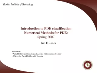
Solving an elliptic PDE using finite differences Numerical Methods for PDEs Spring 2007. Jim E. Jones. Many physical processes can be modeled with Partial Differential Equations (PDEs). Poisson Equation modeling steady-state temperature in 2d plate.

E N D
Solving an elliptic PDE using finite differences Numerical Methods for PDEs Spring 2007 Jim E. Jones
Many physical processes can be modeled with Partial Differential Equations (PDEs) Poisson Equation modeling steady-state temperature in 2d plate Wave Equation modeling wave propagation at speed v Maxwell’s equations relating electric and magnetic fields
Partial Differential Equations (PDEs) :2nd order model problems • PDE classified by discriminant: b2-4ac. • Negative discriminant = Elliptic PDE. Example Laplace’s equation • Zero discriminant = Parabolic PDE. Example Heat equation • Positive discriminant = Hyperbolic PDE. Example Wave equation
Partial Differential Equations (PDEs) :2nd order model problems • PDE classified by discriminant: b2-4ac. • Negative discriminant = Elliptic PDE. Example Laplace’s equation • Zero discriminant = Parabolic PDE. Example Heat equation • Positive discriminant = Hyperbolic PDE. Example Wave equation
Solving PDEs on a computer typically involves discretizing on a grid Computers typically don’t understand continuous quantities, only discrete ones. Rather than asking for the temperature as a function u(x,y), we seek to find an approximation to the temperature at each point on a grid.
Discretization approximates the differential problem by an algebraic one
Finite differences - derived by interpolation (x2,u2) (x1,u1) Construct polynomial interpolating data (xo,u0) x0 x1 x2
Finite differences - derived by Lagrange interpolation (x2,u2) (x1,u1) (xo,u0) Approximate 2nd derivative of u at x1 by 2nd derivative of p x0 x1 x2
Finite differences - derived by Lagrange interpolation (x2,u2) (x1,u1) (xo,u0) h x0 x1 x2
Finite differences - derived by Taylor’s Theorem [Taylor’s Theorem] Suppose f and its first n derivatives are continuous on [a,b], its n+1 derivative exists on [a,b], and xo is in [a,b]. Then for any x in [a,b] there is a c(x) between x and x0 with:
(x2,u2) (x1,u1) (xo,u0) x0 x1 x2 Finite differences
(x2,u2) (x1,u1) (xo,u0) x0 x1 x2 Finite differences
(x2,u2) (x1,u1) (xo,u0) x0 x1 x2 Finite differences If the 4th derivative is continuous, then the average value of u at co and c2 is attained at some c between them. (Intermediate Value Theorem)
(x2,u2) (x1,u1) (xo,u0) x0 x1 x2 Finite differences If the 4th derivative is continuous, then the average value of u at co and c2 is attained at some c between them
(x2,u2) (x1,u1) (xo,u0) x0 x1 x2 Finite differences Solving for u’’
(x2,u2) (x1,u1) (xo,u0) x0 x1 x2 Finite differences Same approximation we got using interpolation Solving for u’’
Finite difference discretization based on Taylor’s approximation.
Finite difference discretization based on Taylor’s approximation. Approximated derivative at a point by an algebraic equation involving function values at nearby points By Taylor’s Theorem, the error in this approximation (the truncation error) is O(h2)
Finite difference discretization based on Taylor’s approximation. Equation for each grid point (x,y) Error in approximation is determined by the mesh size h. Difference between differential solution and algebraic solution goes to zero as h does.
Simple Example on Partial Differential Equation Boundary Conditions on (1,1) (0,0)
Simple Example Where are the discrete u values located?
Simple Example Where are the discrete u values located? At grid points
Simple Example Which u-values do we already know?
Simple Example Which u-values do we already know? The boundary values are =2
Simple Example Write down the 9x9 matrix problem for computing the unknown u-values.
8 9 7 6 4 5 1 3 2 Simple Example Write down the 9x9 matrix problem for computing the unknown u-values.
8 9 7 6 4 5 1 3 2 Linear System
MATLAB • Debugging – does the solution “look correct” • Symmetry • Other checks, can we set it up so we know the solution?
MATLAB • To think about on the MLK Holiday break (and to get ready for assignment 1) • How would you code up the simple example? • How could you allow general mesh size h? • How could you allow general rhs and bc’s? Perhaps even functions that depend on position: sin(xy)? • How would you verify your code is working properly?