Download
1 / 100
1.06k likes | 1.32k Views
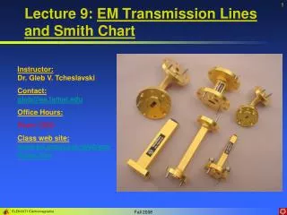
Lecture 9: EM Transmission Lines and Smith Chart. Instructor: Dr. Gleb V. Tcheslavski Contact: gleb@ee.lamar.edu Office Hours: Room 2030 Class web site: www.ee.lamar.edu/gleb/em/Index.htm. Equivalent electrical circuits.

E N D
Lecture 9: EM Transmission Lines and Smith Chart Instructor: Dr. Gleb V. Tcheslavski Contact:gleb@ee.lamar.edu Office Hours: Room 2030 Class web site:www.ee.lamar.edu/gleb/em/Index.htm
Equivalent electrical circuits In this topic, we model three electrical transmission systems that can be used to transmit power: a coaxial cable, a strip line, and two parallel wires (twin lead). Each structure (including the twin lead) may have a dielectric between two conductors used to keep the separation between the metallic elements constant, so that the electrical properties would be constant.
Equivalent electrical circuits Instead of examining the EM field distribution within these transmission lines, we will simplify our discussion by using a simple model consisting of distributed inductors and capacitors. This model is valid if any dimension of the line transverse to the direction of propagation is much less than the wavelength in a free space. The transmission lines considered here support the propagation of waves having both electric and magnetic field intensities transverse to the direction of wave propagation. This setup is sometimes called a transverse electromagnetic (TEM) mode of propagation. We assume no loss in the lines.
Equivalent electrical circuits Distributed transmission line Its equivalent circuit z is a short distance containing the distributed circuit parameter. and are distributed inductance and distributed capacitance. Therefore, each section has inductance and capacitance (9.7.1)
Equivalent electrical circuits (9.8.1) (9.8.2) (9.8.3) Note: the equations for a microstrip line are simplified and do not include effects of fringing. We can model the transmission line with an equivalent circuit consisting of an infinite number of distributed inductors and capacitors.
Equivalent electrical circuits • The following simplifications were used: • No energy loss (resistance) was incorporated; • We neglected parasitic capacitances between the wires that constitute the distributed inductances. We will see later that these parasitic capacitances will lead to changes in phase velocity of the wave (dispersion); • Parameters of the line are constant. We can analyze EM transmission lines either as a large number of distributed two-port networks or as a coupled set of first-order PDEs that are called the telegraphers’ equations.
Transmission line equations While analyzing the equivalent circuit of the lossless transmission line, it is simpler to use Kirchhoff’s laws rather than Maxwell’s equations. Therefore, we will consider the equivalent circuit of this form: For simplicity, we define the inductance and capacitance per unit length: (9.10.1) which have units of Henries per unit length and Farads per unit length, respectively.
Transmission line equations The current entering the node at the location z is I(z). The part of this current will flow through the capacitor, and the rest flows into the section. Therefore: (9.11.1) (9.11.2) , the LHS of (9.11.2) is a spatial derivative. Therefore: (9.11.3)
Transmission line equations Similarly, the sum of the voltage drops in this section can be calculated via the Kirchhoff’s law also: (9.12.1) (9.12.2) , the LHS of (9.12.2) is a spatial derivative. Therefore: (9.12.3)
Transmission line equations The equations (9.11.3) and (9.12.3) are two linear coupled first-order PDEs called the telegrapher’s (Heaviside) equations. They can be composed in a second-order PDE: (9.13.1) (9.13.2) We may recognize that both (9.13.1) and (9.13.2) are wave equations with the velocity of propagation: (9.13.3)
Transmission line equations Example 9.1: Show that a transmission line consisting of distributed linear resistors and capacitors in the given configuration can be used to model diffusion. We assume that the resistance and the capacitance per unit length are defined as (9.14.1) Potential drop over the resistor R and the current through the capacitor C are: (9.14.2) (9.14.3)
Transmission line equations (9.15.1) (9.15.2) The corresponding second-order PDE for the potential is: (9.15.3) Which is a form of a diffusion equation with a diffusion coefficient: (9.15.4)
Transmission line equations Example 9.2: Show that a particular solution for the diffusion equation is given by (9.16.1) Differentiating the solution with respect to z: (9.16.2) (9.16.3) Differentiating the solution with respect to t: (9.16.4)
Transmission line equations Since the RHSs of (9.16.3) and (9.16.4) are equal, the diffusion equation is satisfied. The voltages at different times are shown. The total area under each curve equals 1. This solution would be valid if a certain amount of charge is placed at z = 0 at some moment in the past. Note: the diffusion is significantly different from the wave propagation.
Sinusoidal waves We are looking for the solutions of wave equations (9.13.1) and (9.13.2) for the time-harmonic (AC) case. We must emphasize that – unlike the solution for a static DC case or quasi-static low-frequency case (ones considered in the circuit theory) – these solutions will be in form of traveling waves of voltage and current, propagating in either direction on the transmission line with the velocity specified by (9.13.3). We assume here that the transmission line is connected to a distant generator that produces a sinusoidal signal at fixed frequency = 2f. Moreover, the generator has been turned on some time ago to ensure that transient response decayed to zero; therefore, the line is in a steady-state mode. The most important (and traditional) simplification for the time-harmonic case is the use of phasors. We emphasize that while in the AC circuits analysis phasors are just complex numbers, for the transmission lines, phasors are complex functions of the position z on the line.
Sinusoidal waves (9.19.1) Therefore, the wave equations will become: (9.19.2) (9.19.3) Here, as previously, k isthe wave number: (9.19.4) Velocity of propagation Wavelength of the voltage or current wave
Sinusoidal waves A solution for the wave equation (9.13.3) can be found, for instance, in one of these forms: (9.20.1) (9.20.2) We select the exponential form (9.20.2) since it is easier to interpret in terms of propagating waves of voltage on the transmission line. Example 9.3: The voltage of a wave propagating through a transmission line was continuously measured by a set of detectors placed at different locations along the transmission line. The measured values are plotted. Write an expression for the wave for the given data.
Sinusoidal waves The data Slope of the trajectory…
Sinusoidal waves We assume that the peak-to peak amplitude of the wave is 2V0. We also conclude that the wave propagates in the +z direction. The period of the wave is 2s, therefore, the frequency of oscillations is ½ Hz. (9.22.1) The velocity of propagation can be found from the slope as: (9.22.2) The wave number is: (9.22.3) The wavelength is: (9.22.4) Not in vacuum! Therefore, the wave is: (9.22.5)
Sinusoidal waves Assuming next that the source is located far from the observation point (say, at z = -) and that the transmission line is infinitely long, there would be only a forward traveling wave of voltage on the transmission line. In this case, the voltage on the transmission line is: (9.23.1) The phasor form of (9.12.3) in this case is (9.23.2) Which may be rearranged as: (9.23.3)
Sinusoidal waves The ratio of the voltage to the current is a very important transmission line parameter called the characteristic impedance: (9.24.1) Since (9.24.2) Then: (9.24.3) We emphasize that (9.24.3) is valid for the case when only one wave (traveling either forwards or backwards) exists. In a general case, more complicated expression must be used. If the transmission line was lossy, the characteristic impedance would be complex.
Sinusoidal waves If we know the characteristics of the transmission lane and the forward voltage wave, we may find the forward current wave by dividing voltage by the characteristic impedance. Another important parameter of a transmission line is its length L, which is often normalized by the wavelength of the propagation wave. Assuming that the dielectric between conductors has and
Sinusoidal waves The velocity of propagation does not depend on the dimensions of the transmission line and is only a function of the parameters of the material that separates two conductors. However, the characteristic impedance DOES depend upon the geometry and physical dimensions of the transmission line.
Sinusoidal waves Example 9.4: Evaluate the velocity of propagation and the characteristic impedance of an air-filled coaxial cable with radii of the conductors of 3 mm and 6 mm. The inductance and capacitance per unit length are: (9.27.1) (9.27.2) The velocity of propagation is: (9.27.3) The characteristic impedance of the cable is: (9.27.4) Both the v and the Zc may be decreased by insertion of a dielectric between leads.
Terminators So far, we assumed that the transmission line was infinite. In the reality, however, transmission lines have both the beginning and the end. The line has a real characteristic impedance Zc. We assume that the source of the wave is at z = - and the termination (the end of the line) is at z = 0. The termination may be either an impedance or another transmission line with different parameters. We also assume no transients.
Terminators The phasor voltage at any point on the line is: (9.29.1) The phasor current is: (9.29.2) At the load location (z = 0), the ratio of voltage to current must be equal ZL: (9.29.3) Note: the ratio B2 to A2 represents the magnitude of the wave incident on the load ZL.
Terminators We introduce the reflection coefficient for the transmission line with a load as: (9.30.1) Often, the normalized impedance is used: (9.30.2) The reflection coefficient then becomes: (9.30.3)
Terminators Therefore, the phasor representations for the voltage and the current are: (9.31.1) (9.31.2) The total impedance is: (9.31.3) generally a complicated function of the position and NOT equal to Zc. However, a special case of matched load exists when: (9.31.4) In this situation: (9.31.5)
Terminators Example 9.5: Evaluate the reflection coefficient for a wave that is incident from z = - in an infinitely long coaxial cable that has r = 2 for z < 0 and r = 3 for z > 0. The characteristic impedance is: The load impedance of a line is the characteristic impedance of the line for z > 0.
Terminators The reflection coefficient can be expressed as:
Terminators The reflection coefficient is completely determined by the value of the impedance of the load and the characteristic impedance of the transmission line. The reflection coefficient for a lossless transmission line can have any complex value with magnitude less or equal to one. If the load is a short circuit (ZL = 0), the reflection coefficient = -1. The voltage at the load is a sum of voltages of the incident and the reflected components and must be equal to zero since the voltage across the short circuit is zero. If the load is an open circuit (ZL = ), the reflection coefficient = +1. The voltage at the load can be arbitrary but the total current must be zero. If the load impedance is equal to the characteristic impedance (ZL = Zc), the reflection coefficient = 0 – line is matched. In this case, all energy of generator will be absorbed by the load.
Terminators For the shorten transmission line: (9.35.1) (9.35.2) For the open transmission line: (9.35.3) (9.35.4) In both cases, a standing wave is created. The signal does not appear to propagate.
Terminators Since the current can be found as ZL = 0 ZL = Note that the current wave differs from the voltage wave by 900
Terminators Another important quantity is the ratio of the maximum voltage to the minimum voltage called the voltage standing wave ratio: (9.37.1) Which leads to (9.37.2) VSWR, the reflection coefficient, the load impedance, and the characteristic impedance are related. Even when the amplitude of the incident wave V0 does not exceed the maximally allowed value for the transmission line, reflection may lead to the voltage V0(1+||) exceeding the maximally allowed. Therefore, the load and the line must be matched.
Terminators Example 9.6: Evaluate the VSWR for the coaxial cable described in the Example 9.5. The reflection coefficient was evaluated as = -0.1. Note: if two cables were matched, the VSWR would be 1.
Impedance and line matching The ratio of total phasor voltage to total phasor current on a transmission line has units of impedance. However, since both voltage and current consist of the incident and reflected waves, this impedance varies with location along the line. (9.40.1) Incorporating (9.30.1), we obtain: (9.40.2) The last formula is most often used to find the impedance at the line terminals.
Impedance and line matching Considering the transmission line shown, we assume that a load with the impedance ZL is connected to a transmission line of length L having the characteristic impedance Zc and the wave number k. The input impedance can be found as an impedance at z = -L: (9.41.1) Or as the normalized input impedance: (9.41.2)
Impedance and line matching (Ex) Example 9.7: A signal generator whose frequency f = 100 MHz is connected to a coaxial cable of characteristic impedance 100 and length of 100 m. The velocity of propagation is 2108 m/s. The line is terminated with a load whose impedance is 50 . Calculate the impedance at a distance 50 m from the load. The normalized load impedance is The wave number is The normalized input impedance is Therefore, the input impedance is
Impedance and line matching The wave number can be expressed in terms of wavelength: (9.43.1) Therefore: (9.43.2) and (9.43.3) If the length of the transmission line is one quarter of a wavelength, (9.43.4) tangent (9.42.3) approaches infinity and (9.43.5) Implying that the normalized input impedance zin of a /4 line terminated with the load ZL is numerically equal to the normalized load admittanceyL = 1/zL.
Impedance and line matching The last example represents a one quarter-wavelength transmission line that is useful in joining two transmission lines with different characteristic impedances or in matching a load. One of the simplest matching techniques is to use a quarter-wave transformer – a section of a transmission line that has a particular characteristic impedance Zc(/4). This characteristic impedance Zc(/4) must be chosen such that the reflection coefficient at the input of the matching transmission line section is zero. This happens when (9.44.1) One considerable disadvantage of this method is its frequency dependence since the wavelength depends on the frequency.
Impedance and line matching When the load impedance equals the characteristic impedance, the load and the line are matched and no reflection of the wave occurs. For the short circuit and the open circuit: (9.45.1) (9.45.2) In practice, it is easier to make short circuit terminators since fringing effects may exist in open circuits. In both cases, the input impedance will be a reactance, Zin = jXin as shown for a short-circuited (a) and an open-circuited (b) transmission lines. The value of the impedance depends on the length of the transmission line, which implies that we can observe/have any possible value of reactance that is either capacitive or inductive.
Impedance and line matching Types of input impedance of short-circuited and open-circuited lossless transmission lines: We introduce the characteristic admittance of the transmission line: (9.46.1) and the input susceptance of the transmission line: (9.46.2)
Impedance and line matching Assuming that a transmission line is terminated with a load impedance ZL or load admittance YL that is not equal to the line’s characteristic admittance Yc. Let the input admittance of the line be Yc + jB at the distance d1 from the load. If, at this distance d1, we connect a susceptance –jB in parallel to the line, the total admittance to the left of this point (d1) will be Yc. The transmission line is matched from the insertion point (d1) back to the generator. In practice, matching can be done by insertion of a short-circuited transmission line of particular length.
Impedance and line matching Such transmission line used to match another (main) transmission line is called a stub. The length of a stub is chosen to make its admittance be equal –jB. This process of line matching is called single-stub matching. The length of the stub can be made adjustable. Such adjustable-length transmission lines are sometimes called a trombone line. Note that single-stub matching requires two adjustable distances: location of the stub d1 and the length of the stub d2. In some situations, only the stub’s length can be adjusted. In these cases, additional stub(s) may be used. The distances mentioned here are normalized to the wavelength. Therefore, this method allows line matching at particular discrete frequencies.
Impedance and line matching (Ex) Example 9.8: A lossless transmission line is terminated with an impedance whose value is a half of the characteristic impedance of the line. What impedance should be inserted in parallel with the load at the distance /4 from the load to minimize the reflection from the load? To minimize the reflection, the parallel combination of the ZQ and the input impedance at that location should equal to the characteristic impedance of the line.
Smith chart The input impedance of a transmission line depends on the impedance of the load, the characteristic impedance of the line, and the distance between the load and the observation point. The value of the input impedance also periodically varies in space. The input impedance can be found graphically via so called Smith chart. The normalized impedance at any location is complex and can be found as: (9.50.1) An arbitrary normalized load impedance is: (9.50.2) Where: (9.50.3) Since the line is assumed to be lossless, its characteristic impedance is real.