Open Universe State Estimation with DBLOG: A Comparative Analysis
Learn how DBLOG revolutionizes data association methods by instantiating all hypothesized sources, addressing the disparity with ad hoc solutions, and enabling advanced modeling techniques for state estimation. Discover the key differences, challenges, and benefits of DBLOG in state inference processes.

Open Universe State Estimation with DBLOG: A Comparative Analysis
E N D
Presentation Transcript
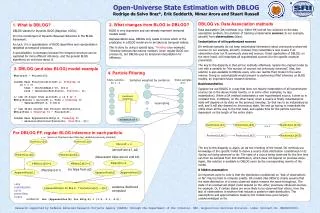
* Open-Universe State Estimation with DBLOG Rodrigo de Salvo Braz*, Erik Sudderth, Nimar Arora and Stuart Russell DBLOG vs. Data Association methods Data Association (DA) methods (e.g. Sittler '64) are ad hoc solutions to the data association problem, the problem of tracking unobservable sources (in our example, aircraft) from observations (blips). Instantiation of all hypothesized sources DA methods typically do not keep instantiated information about previously unobserved sources (in our example, aircraft). Instead, they instantiate a new source if an observation does not fit previously observed sources. Direct application of DBLOG, on the other hand, will instantiate all hypothesized sources (for the specific example presented). The key to this disparity is that ad hoc methods effectively replace the original model by one with a variable for “the number of sources not previously observed”. Alas, this solution is also available to DBLOG users, who can rewrite their model in the same manner. Doing so automatically would amount to performing lifted inference on BLOG models, an important future research direction. Backinstantiation Suppose we use DBLOG in a way that does not require instantiation of all hypothesized sources (as in the above model rewrite, or in some other examples, by lazy instantiation). When a DA method instantiates a new hypothesized source, it does so in constant time. In DBLOG, on the other hand, when a source is finally instantiated its state will depend on its state on the previous timestep. So that has to be instantiated as well, and it will also depend on its previous state. We end up having to instantiate the entire chain all the way to the first state, and update time for the particle becomes dependent on the length of the entire chain. The key to this disparity is, again, an ad hoc rewriting of the model. DA methods use knowledge of the specific model to derive a source state distribution conditioned on its having not being observed so far. The state of a source being observed for the first time can then be sampled from that distribution, which does not depend on previous steps. Again, this solution is available to DBLOG users by the corresponding rewrite of the model. A hidden assumption An important point to note is that the distribution conditioned on “lack of observations so far” may be hard to compute exactly. DA models (like Sittler’s) simply assume that the state distribution of a newly observed object remains the same throughout. The state of an unobserved object could depend on the other, previously observed sources, for example. Or, if certain states are more likely to be observed than others, then the lack of observations is evidence that induces a posterior state distribution. The assumptions and approximations made by DA models have gone largerly unacknowledged so far. 2. What changes from BLOG to DBLOG? BLOG is very expressive and can already represent temporal models easily. Representation-wise, DBLOG only needs to know which of the predicates in a BLOG model are to be taken as temporal indices. This is done by using a special type, Timestep (see example). Timestep behaves like natural numbers (even regular BLOG can process it), but DBLOG uses its temporal interpretation for efficiency. 1. What is DBLOG? DBLOG stands for Dynamic BLOG (Bayesian LOGic). It is the counterpart of Dynamic Bayesian Networks in the BLOG framework. As such, it is a specialization of BLOG algorithms and representation targetted at temporal processes. A specialization is necessary because the temporal structure can be exploited for more efficient inference, and the general BLOG algorithms do not know about it. 3. DBLOG (and also BLOG) model example #Aircraft ~ Poisson[3]; random Real Position(Aircraft a, Timestep t) if t = @1 then ~ UniformReal[-10, 10]() else ~ Gaussian(Position(a, Prev(t)), 2); // num of blips from aircraft a is 0 or 1 #Blip(Source = Aircraft a, Time = Timestep t) ~ TabularCPD[[0.2, 0.8]]() // num false alarms has Poisson distribution. #Blip(Time = Timestep t) ~ Poisson[2]; random Real ApparentPos(Blip b, Timestept) ~ Gaussian(Position(Source(b), Prev(t)), 2)); 4. Particle Filtering State samples for t - 1 Samples weighed by evidence State samples for t Likelihoodweighting resampling evidence at t ... Position(a1,@1) Position(a1,@2) Position(a1,@15) For DBLOG PF, regular BLOG inference in each particle ... ... (previous timesteps have their own variables previously sampled) Position(a2,@1) Position(a2,@2) Position(a2,@15) Position(a1,@1) Position(a2,@1) #Aircraft = 2 (aircraft are a1, a2) Position(a1,@2) Position(a2,@2) (false alarm blips are b2 and b3) #Blip(@2)=2 #Blip(a1,@2)=1 #Blip(a2,@2)=0 (no blips from a2) (this blip is b1) ApparentPos(b1) ApparentPos(b2) ApparentPos(b3) Lazy instantiation up to parentless nodes {ApparentPos(b) for Blip b : Time(Source(b)) = @2} evidence likelihood computed evidence: obs {ApparentPos(b) for Blip b} = {1.2, 3.1, 4.0}; Research supported by Defense Advanced Research Projects Agency (DARPA) through the Department of the Interior, NBC, Acquisition Services Division, under Contract No. NBCHD030010.

