Confounding and Interaction: Part III

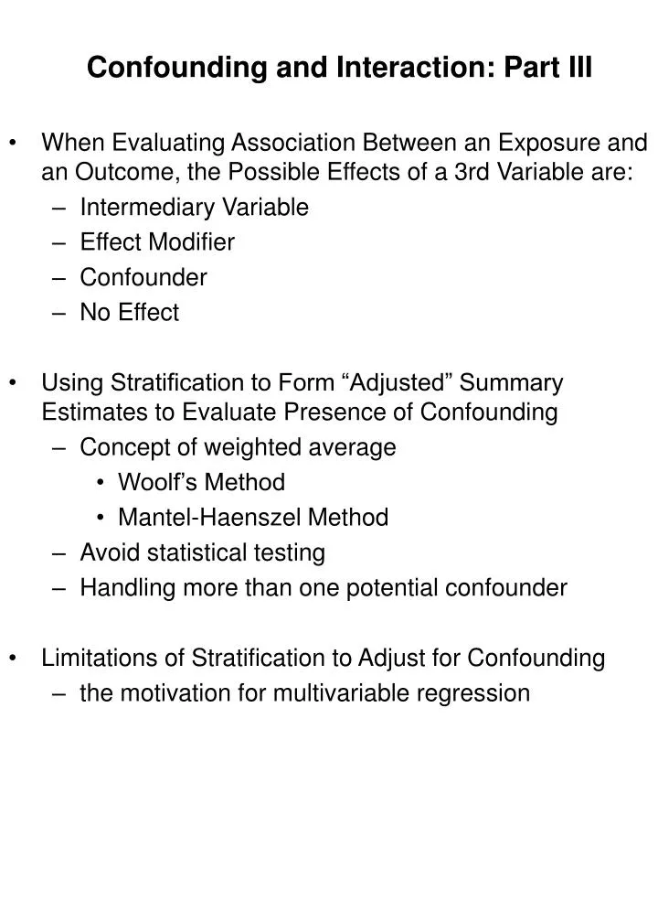
1. Confounding and Interaction: Part III • When Evaluating Association Between an Exposure and an Outcome, the Possible Effects of a 3rd Variable are: • Intermediary Variable • Effect Modifier • Confounder • No Effect • Using Stratification to Form “Adjusted” Summary Estimates to Evaluate Presence of Confounding • Concept of weighted average • Woolf’s Method • Mantel-Haenszel Method • Avoid statistical testing • Handling more than one potential confounder • Limitations of Stratification to Adjust for Confounding • the motivation for multivariable regression

2. When Assessing the Association Between an Exposure and a Disease, What are the Possible Effects of a Third Variable? No Effect + C Intermediary Variable I Effect Modifier _ Interaction: MODIFIES THE EFFECT OF THE EXPOSURE Confounding: ANOTHER PATHWAY TO GET TO THE DISEASE D

3. What are the Possible Effects of a 3rd Variable? • Intermediary Variable • Effect Modifier (interaction) • Confounder • No Effect Intermediary Variable (conceptual decision)? Report Crude Estimate no yes Effect Modifier? no yes Report stratum-specific estimates Confounder? No Effect: Report Crude Estimate Report “adjusted” summary estimate no yes

4. Interaction with a Third Variable Crude RR crude= 1.7 Stratified Heavy Caffeine Use No Caffeine Use RRcaffeine use = 0.7 RRnocaffeine use = 2.4

5. Is Interaction Present? • Does the relationship between the exposure and the outcome vary meaningfully (in a clinical/biologic sense) across strata of the third variable? • Does an average (adjusted) effect (formed by averaging the strata formed on the basis of the third variable) reasonably represent all strata? • if yes, go on to form an average (adjusted) measure • if no, stop - this is interaction; report stratum-specific estimates

6. Declare vs Ignore Interaction?

7. No Effect of Third Variable Crude ORcrude = 21.0 (95% CI: 16.4 - 26.9) Stratified Matches Present Matches Absent ORmatches = 21.0 OR nomatches = 21.0 ORadj= 21.0 (95% CI: 14.2 - 31.1)

8. Confounding by Third Variable Crude ORcrude = 8.8 Stratified Smokers Non-Smokers ORsmokers = 1.0 OR non-smokers = 1.0 OR adj = 1.0

9. Forming an Adjusted Summary Estimate Crude OR crude = 3.5 Stratified Age < 35 Age > 35 ORage <35 = 3.4 ORage >35 = 5.7 Test of homogeneity: p = 0.71

10. Assuming Interaction is not Present, Form a Summary of the Unconfounded Stratum-Specific Estimates Right. We need to assign a weight to each stratum and then perform a weighted average. • Construct a weighted average • Assign weights to the individual strata • Summary Estimate = Weighted Average of the stratum-specific estimates • a simple mean is a weighted average where the weights are equal to 1 • which weights to use depends on type of effect estimate desired (OR, RR, RD) and characteristics of the data • e.g. • Woolf’s method • Mantel-Haenszel method Hopefully the concept of a weighted average is understood by everyone. A simple mean is in fact a weighted average where the weights equal one. To get the average height of everyone in class, we add up everyone’s height and divide by the number of persons contributing. The weight is one. How do we decide on a weight? The second approach to getting a summary estimate is actually the one used by multivariable modeling approaches and we will touch on this briefly today. It is called the maximum likelihood approach

11. Forming a Summary Estimate for Stratified Data After we have formed our strata and gotten rid of confounding, how do we summarize what the unconfounded estimates from the two or more strata are telling us. In the examples of last week, the measures of association from the different strata were identical. This is seldom the case. • Goal: • Create a summary “adjusted” estimate for the relationship in question while adjusting for the potential confounder • e.g.: • Case-control study of post-exposure AZT use in preventing HIV seroconversion after needlestick (NEJM 1997) A more realistic is described in the Rothman chapter regarding the question of whether spermicide use might cause Down’s Crude ORcrude =0.61 (95% CI: 0.26 - 1.4) The goal is to combine or average the results from the different strata into one summary estimate. Any thoughts on how to do this?

12. Post-exposure prophylaxis with AZT after a needlestick AZT Use Severity of Exposure HIV

13. Forming a Summary Estimate for Stratified Data After we have formed our strata and gotten rid of confounding, how do we summarize what the unconfounded estimates from the two or more strata are telling us. In the examples of last week, the measures of association from the different strata were identical. This is seldom the case. • Potential confounder: severity of exposure Crude A more realistic is described in the Rothman chapter regarding the question of whether spermicide use might cause Down’s ORcrude =0.61 Stratified Minor Severity Major Severity OR = 0.0 OR = 0.35 The goal is to combine or average the results from the different strata into one summary estimate. Any thoughts on how to do this?

14. To stratify the subjects into those women with maternal age less than 35 and those with maternal age >= 35, you add a “by(matage) option. If you add a “, pool” option as I have here, the program will give you not only the default MH summary but also the Woolf estimate. Finally, you are already familiar with this command but for sake of comparison let’s look at the summary estimate as obtained by logistic regression which as you know uses the MLE approach. As you can see, the MH estimate is essentially identical to the MLE in this problem.

15. Forming a Summary Estimate for Stratified Data After we have formed our strata and gotten rid of confounding, how do we summarize what the unconfounded estimates from the two or more strata are telling us. In the examples of last week, the measures of association from the different strata were identical. This is seldom the case. • Goal: • Create a summary “adjusted” estimate for the relationship in question while adjusting for the potential confounder • e.g.: • AZT use, severity of needlestick and HIV seroconversion after needlestick (NEJM 1997) A more realistic is described in the Rothman chapter regarding the question of whether spermicide use might cause Down’s Crude ORcrude =0.61 Stratified Minor Severity Major Severity OR = 0.0 OR = 0.35 The goal is to combine or average the results from the different strata into one summary estimate. Any thoughts on how to do this?

16. Summary Estimators: Woolf’s Method One of the first approaches developed for forming summaryl adjusted estimates was Woolf’s method: • aka Directly pooled or precision estimator • Woolf’s estimate for odds ratio • where wi • wi is the inverse of the variance of the stratum-specific log(odds ratio) This is the inverse of the variance of the log odds ratio. This makes sense the more precise strata have the smallest variances and the inverse of a small number is a large number

17. Calculating a Summary Effect Using the Woolf Estimator After we have formed our strata and gotten rid of confounding, how do we summarize what the unconfounded estimates from the two or more strata are telling us. In the examples of last week, the measures of association from the different strata were identical. This is seldom the case. • e.g. AZT use, severity of needlestick, and HIV Crude ORcrude =0.61 A more realistic is described in the Rothman chapter regarding the question of whether spermicide use might cause Down’s Stratified Minor Severity Major Severity OR = 0.0 OR = 0.35 The goal is to combine or average the results from the different strata into one summary estimate. Any thoughts on how to do this?

18. Summary Estimators: Woolf’s Method I discuss this approach first not only because it was one of the first proposed but also because it is the most conceptually straightforward. • Conceptually straightforward although computationally messy • Best when: • number of strata is small • sample size within each strata is large • Cannot be calculated when any cell in any stratum is zero because log(0) is undefined • 1/2 cell corrections have been suggested but are subject to bias • Formulae for Woolf’s summary estimates for other measures (RR, RD, AR) available in texts and software documentation • sensitive to small strata, cells with “0” • computationally messy It seems the most reasonable to assign each stratum according to how sure you are of the inference and the variance of the estimate is the best measure we have for this. In the days before computers, this was considered computationally messy such that other easier methods were sought

19. A more robust approach is the Mantel-Haenszel method Summary Estimators: Mantel-Haenszel Again, using the same cell definitions, the M-H estimate for the summary OR is the sum of a times d divided by T divided by the sum of . . . • Mantel-Haenszel estimate for odds ratios • ORMH = • wi = • wi is inverse of the variance of the stratum-specific odds ratio under the null hypothesis (OR =1) If we decompose this slightly, we can see that the weight is for each stratum is actually b times c divided by T. This is actually the inverse of the . . . And the same logic as before, strata with the smallest variance get the most weight

20. Summary Estimators: Mantel-Haenszel The MH is the most commonly used estimator. • Mantel-Haenszel estimate for odds ratios • resistant to the effects of large numbers of strata with few observations • resistant to cells with a value of “0” • computationally easy • most commonly used It is fairly resistant (ie it doesn’t blow up) . . . Although really not a factor in the computer era, the computation of the MH estimator is a breeze. More importantly is that the M-H closely approximates the MLE estimate which is generally regarded as the most accurate.

21. Calculating a Summary Effect Using the Mantel-Haenszel Estimator After we have formed our strata and gotten rid of confounding, how do we summarize what the unconfounded estimates from the two or more strata are telling us. In the examples of last week, the measures of association from the different strata were identical. This is seldom the case. • e.g. AZT use, severity of needlestick, and HIV • ORMH = • ORMH = Crude ORcrude =0.61 A more realistic is described in the Rothman chapter regarding the question of whether spermicide use might cause Down’s Stratified Minor Severity Major Severity OR = 0.0 OR = 0.35 The goal is to combine or average the results from the different strata into one summary estimate. Any thoughts on how to do this?

22. How can we make our lives a lot easier and implement all of this on the computer? Calculating a Summary Effect in Stata The epitab command - Tables for Epidemiologists is quite a little handy command. Has anyone used it ? • epitab command - Tables for epidemiologists • see Reference manual A-G • To produce crude estimates and 2 x 2 tables: • For cross-sectional or cohort studies: • cs variablecase variable exposed • For case-control studies: • cc variablecase variableexposed • To stratify by a third variable: • cs varcase varexposed, by(varthird variable) • cc varcase varexposed, by(varthird variable) • Default summary estimator is Mantel-Haenszel • , pool will also produce Woolf’s method

23. Calculating a Summary Effect Using the Mantel-Haenszel Estimator After we have formed our strata and gotten rid of confounding, how do we summarize what the unconfounded estimates from the two or more strata are telling us. In the examples of last week, the measures of association from the different strata were identical. This is seldom the case. • e.g. AZT use, severity of needlestick, and HIV • . cc HIV AZTuse,by(severity) pool • severity | OR [95% Conf. Interval] M-H Weight • -----------------+------------------------------------------------- • minor | 0 0 2.302373 1.070588 • major | .35 .1344565 .9144599 6.956522 • -----------------+------------------------------------------------- • Crude | .6074729 .2638181 1.401432 • Pooled (direct) | . . . • M-H combined | .30332 .1158571 .7941072 • -----------------+------------------------------------------------- • Test of homogeneity (B-D) chi2(1) = 0.60 Pr>chi2 = 0.4400 • Test that combined OR = 1: • Mantel-Haenszel chi2(1) = 6.06 • Pr>chi2 = 0.0138 Crude ORcrude =0.61 A more realistic is described in the Rothman chapter regarding the question of whether spermicide use might cause Down’s Stratified Minor Severity Major Severity OR = 0.0 OR = 0.35 The goal is to combine or average the results from the different strata into one summary estimate. Any thoughts on how to do this?

24. Calculating a Summary Effect Using the Mantel-Haenszel Estimator • In addition to the odds ratio, Mantel-Haenszel estimators are also available in Stata for: • risk ratio • “cs varcase varexposed, by(varthird variable)” • or st stir • rate ratio • “ir varcase varexposed vartime, by(varthird variable)” • or st strate

25. Mantel-Haenszel Confidence Interval and Hypothesis Testing

26. Mantel-Haenszel Techniques • Mantel-Haenszel estimators • Mantel-Haenszel chi-square statistic • Mantel’s test for trend (dose-response)

27. Assessment of Confounding: Interpretation of Summary Estimate If the summary estimate, here a M-H OR estimator of 3.8 • Compare “adjusted” summary estimate to crude estimate • e.g. compare ORMH (= 0.30 in the example) to ORcrude (= 0.61 in the example) • If “adjusted” measure “differs meaningfully” from crude estimate, then confounding is present • e.g., does ORMH = 0.30 “differ meaningfully” from ORcrude = 0.61? • What does “differs meaningfully” mean? • a matter of judgement based on biologic/clinical sense rather than on a statistical test • no one correct answer • 10% change often used • your threshold needs to be stated a priori and included in your methods section So, its in the hands of the researcher

28. Summary Effect in Stata -example • e.g. Spermicide use, maternal age and Down’s With this in mind, let’s consider an example using . . . Crude OR = 3.5 Age < 35 Age > 35 Stratified OR = 3.4 OR = 5.7 Should we pool these? Is there confounding present?

29. Presence or Absence of Confounding by a Third Variable?

30. Statistical Testing for Confounding is Inappropriate • Testing for statistically significant differences between crude and adjusted measures is inappropriate • e.g. when examining an association for which a factor is a known confounder (say age in the association between HTN and CAD) • if the study has a small sample size, even large differences between crude and adjusted measures will not be statistically different • yet, we know confounding is present • therefore, the difference between crude and adjusted measures cannot be ignored as merely chance and must be reported as confounding

31. Statistical Testing for Confounding is Inappropriate • Furthermore, with large sample sizes, even factors which truly are not confounders can appear to cause confounding that is “statistically significant” • e.g., study of sunlight exposure and melanoma • prior knowledge: no relationship between gum chewing and melanoma • data: gum chewing is assoc. with sunlight exposure and with melanoma and adjusted measure of association is statistically different than the crude association? • should gum chewing be controlled for? • To resolve this paradox, only adjust for factors for which you have biologic rationale (i.e., some prior probability)

32. Stratification - Effect of Excessive Correlation Between Exposure & Confounder After we have formed our strata and gotten rid of confounding, how do we summarize what the unconfounded estimates from the two or more strata are telling us. In the examples of last week, the measures of association from the different strata were identical. This is seldom the case. • e.g. race/SES; income/education; no. of sexual partners/no. of anal intercourse partners • aka collinearity • precludes ability to adjust A more realistic is described in the Rothman chapter regarding the question of whether spermicide use might cause Down’s Crude RRcrude =8.0 Stratified Low Education High Education RR = undefined RR = 12.5 The goal is to combine or average the results from the different strata into one summary estimate. Any thoughts on how to do this?

33. When More than One Additional Variable is Present Crude Stratified white smokers black smokers latino smokers white non-smokers black non-smokers latino non-smokers

34. The Need for Evaluation of Joint Confounding The examples I have shown thus far have just one potential confounder to worry about. What should we do when more than . . . • Variables that evaluated alone show no confounding may show confounding when evaluated jointly Crude Stratified by Factor 1 by Factor 2 by Factor 1 & 2 In this example, the crude estimate is identical to the stratum specific measures when the 2 other variables are looked at separately.

35. Approaches for When More than One Potential Confounder is Present This introduces the whole topic of • Backward versus forward confounder evaluation strategies • relevant both for stratification and especially multivariable modeling • Backwards Strategy • initially evaluate all potential confounders together (look for joint confounding) • conceptually preferred because in nature variables are all present and act together • Procedure: • with all potential confounders considered, form adjusted estimate • one variable can then be dropped and the adjusted estimate is re-calculated (adjusted for remaining variables) • if the dropping of the first variable results in an inconsequential change, it can be eliminated • procedure continues until no more variables can be dropped • Problem: • with many potential confounders, cells become very sparse and strata very imprecise I know you are learning a bit about this in biostatistics. Which is preferable -backward or forwards? In fact, you may not even be able to get off the ground because the initial stratification is just too thin

36. Approaches for When More than One Potential Confounder is Present In the forward selection approach, you start with . . . • Forward Strategy • start with the variable that has the biggest “change-in-estimate” impact • then add the variable with the second biggest impact • keep this variable if its presence meaningfully changes the adjusted estimate • procedure continues until no other added variable has an important impact • Advantage: • avoids the initial sparse cell problem of backwards approach • Problem: • does not evaluate joint confounding effects of many variables

37. Stratification to Reduce Confounding Although you are all now learning about the wonderful world of multivariable modeling, I would encourage you to examine your data whenever you can with stratification because it is the most native way to see your data and the easiest to explain your data to others • Advantages • straightforward to implement and comprehend • easy to evaluate interaction • Limitations • Looks at only one exposure-disease assoc. at a time • Requires continuous variables to be discretized • loses information; possibly results in “residual confounding” • Deteriorates with multiple confounders • e.g. suppose 4 confounders with 3 levels • 3x3x3x3=81 strata needed • unless huge sample, many cells have “0”’s and strata have undefined effect measures • Solution: • Mathematical modeling (multivariable regression) • e.g. • linear regression • logistic regression • proportional hazards regression It does, however, have its limitations which is principally that it breaks down with multiple confounders These approaches are the topics of Mitch Katz’s upcoming sessions and your Thursday sessions.